Surfaces

Common surfaces

A number of utility functions are provided to set up the most common surfaces, to add vacuum layers, and to add adsorbates to a surface. In general, all surfaces can be set up with the modules described in the section General crystal structures and surfaces, but these utility functions make common tasks easier.

Example

To setup an Al(111) surface with a hydrogen atom adsorbed in an on-top position:

from ase.build import fcc111
slab = fcc111('Al', size=(2,2,3), vacuum=10.0)

This will produce a slab 2x2x3 times the minimal possible size, with a (111) surface in the z direction. A 10 Å vacuum layer is added on each side.

To set up the same surface with with a hydrogen atom adsorbed in an on-top position 1.5 Å above the top layer:

from ase.build import fcc111, add_adsorbate
slab = fcc111('Al', size=(2,2,3))
add_adsorbate(slab, 'H', 1.5, 'ontop')
slab.center(vacuum=10.0, axis=2)

Note that in this case it is probably not meaningful to use the vacuum keyword to fcc111, as we want to leave 10 Å of vacuum after the adsorbate has been added. Instead, the center() method of the Atoms is used to add the vacuum and center the system.

The atoms in the slab will have tags set to the layer number: First layer atoms will have tag=1, second layer atoms will have tag=2, and so on. Adsorbates get tag=0:

>>> print(atoms.get_tags())
[3 3 3 3 2 2 2 2 1 1 1 1 0]

This can be useful for setting up ase.constraints (see Surface diffusion energy barriers using the Nudged Elastic Band (NEB) method).

Utility functions for setting up surfaces

All the functions setting up surfaces take the same arguments.

symbol:

The chemical symbol of the element to use.

size:

A tuple giving the system size in units of the minimal unit cell.

a:

(optional) The lattice constant. If specified, it overrides the expermental lattice constant of the element. Must be specified if setting up a crystal structure different from the one found in nature.

c:

(optional) Extra HCP lattice constant. If specified, it overrides the expermental lattice constant of the element. Can be specified if setting up a crystal structure different from the one found in nature and an ideal \(c/a\) ratio is not wanted (\(c/a=(8/3)^{1/2}\)).

vacuum:

The thickness of the vacuum layer. The specified amount of vacuum appears on both sides of the slab. Default value is None, meaning not to add any vacuum. In that case the third axis perpendicular to the surface will be undefined ([0, 0, 0]) or left at its intrinsic bulk value if requested (see periodic). Some calculators can work with undefined axes as long as the pbc flag is set to False along that direction.

orthogonal:

(optional, not supported by all functions). If specified and true, forces the creation of a unit cell with orthogonal basis vectors. If the default is such a unit cell, this argument is not supported.

periodic:

(optional) Produce a bulk system. Defaults to False. If true, sets boundary conditions and cell constantly with the corresponding bulk structure. Useful for stacking multiple different surfaces. The system will be fully equivalent to the bulk material only if the number of layers is consistent with the crystal stacking.

Each function defines a number of standard adsorption sites that can later be used when adding an adsorbate with ase.build.add_adsorbate().

The following functions are provided

ase.build.fcc100(symbol, size, a=None, vacuum=None, orthogonal=True, periodic=False)

FCC(100) surface.

Supported special adsorption sites: ‘ontop’, ‘bridge’, ‘hollow’.

ase.build.fcc110(symbol, size, a=None, vacuum=None, orthogonal=True, periodic=False)

FCC(110) surface.

Supported special adsorption sites: ‘ontop’, ‘longbridge’, ‘shortbridge’, ‘hollow’.

ase.build.bcc100(symbol, size, a=None, vacuum=None, orthogonal=True, periodic=False)

BCC(100) surface.

Supported special adsorption sites: ‘ontop’, ‘bridge’, ‘hollow’.

ase.build.hcp10m10(symbol, size, a=None, c=None, vacuum=None, orthogonal=True, periodic=False)

HCP(10m10) surface.

Supported special adsorption sites: ‘ontop’.

Works only for size=(i,j,k) with j even.

ase.build.diamond100(symbol, size, a=None, vacuum=None, orthogonal=True, periodic=False)

DIAMOND(100) surface.

Supported special adsorption sites: ‘ontop’.

These always give orthorhombic cells:

fcc100
fcc110
bcc100
hcp10m10
diamond100

ase.build.fcc111(symbol, size, a=None, vacuum=None, orthogonal=False, periodic=False)

FCC(111) surface.

Supported special adsorption sites: ‘ontop’, ‘bridge’, ‘fcc’ and ‘hcp’.

Use orthogonal=True to get an orthogonal unit cell - works only for size=(i,j,k) with j even.

ase.build.fcc211(symbol, size, a=None, vacuum=None, orthogonal=True)

FCC(211) surface.

Does not currently support special adsorption sites.

Currently only implemented for orthogonal=True with size specified as (i, j, k), where i, j, and k are number of atoms in each direction. i must be divisible by 3 to accommodate the step width.

ase.build.bcc110(symbol, size, a=None, vacuum=None, orthogonal=False, periodic=False)

BCC(110) surface.

Supported special adsorption sites: ‘ontop’, ‘longbridge’, ‘shortbridge’, ‘hollow’.

Use orthogonal=True to get an orthogonal unit cell - works only for size=(i,j,k) with j even.

ase.build.bcc111(symbol, size, a=None, vacuum=None, orthogonal=False, periodic=False)

BCC(111) surface.

Supported special adsorption sites: ‘ontop’.

Use orthogonal=True to get an orthogonal unit cell - works only for size=(i,j,k) with j even.

ase.build.hcp0001(symbol, size, a=None, c=None, vacuum=None, orthogonal=False, periodic=False)

HCP(0001) surface.

Supported special adsorption sites: ‘ontop’, ‘bridge’, ‘fcc’ and ‘hcp’.

Use orthogonal=True to get an orthogonal unit cell - works only for size=(i,j,k) with j even.

ase.build.diamond111(symbol, size, a=None, vacuum=None, orthogonal=False, periodic=False)

DIAMOND(111) surface.

Supported special adsorption sites: ‘ontop’.

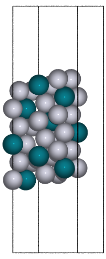
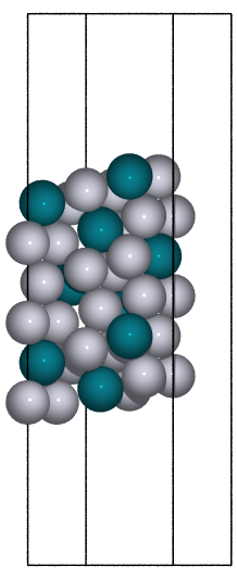
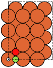
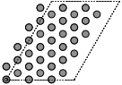
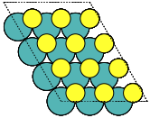
These can give both non-orthorhombic and orthorhombic cells:

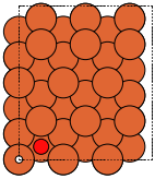
fcc111
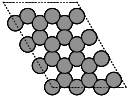
fcc211	not implemented
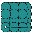
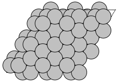
bcc110
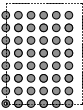
bcc111
hcp0001
diamond111		not implemented

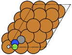
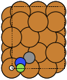
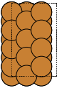
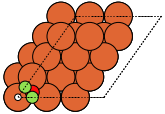
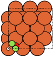
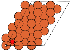
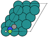
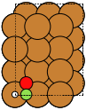
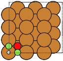
The adsorption sites are marked with:

ontop	hollow	fcc	hcp	bridge	shortbridge	longbridge

ase.build.mx2(formula='MoS2', kind='2H', a=3.18, thickness=3.19, size=(1, 1, 1), vacuum=None)

Create three-layer 2D materials with hexagonal structure.

This can be used for e.g. metal dichalcogenides MX₂ 2D structures such as MoS₂.

https://en.wikipedia.org/wiki/Transition_metal_dichalcogenide_monolayers

Parameters:

kind ({'2H', '1T'}, default: '2H') –

• ‘2H’: mirror-plane symmetry

• ’1T’: inversion symmetry

ase.build.graphene(formula='C2', a=2.46, thickness=0.0, size=(1, 1, 1), vacuum=None)

Create a graphene monolayer structure.

Parameters:

thickness (float, default: 0.0) – Thickness of the layer; maybe for a buckled structure like silicene.

Create root cuts of surfaces

To create some more complicated cuts of a standard surface, a root cell generator has been created. While it can be used for arbitrary cells, some more common functions have been provided.

ase.build.fcc111_root(symbol, root, size, a=None, vacuum=None, orthogonal=False)

FCC(111) surface maniupulated to have a x unit side length of root before repeating. This also results in root number of repetitions of the cell.

The first 20 valid roots for nonorthogonal are… 1, 3, 4, 7, 9, 12, 13, 16, 19, 21, 25, 27, 28, 31, 36, 37, 39, 43, 48, 49

ase.build.hcp0001_root(symbol, root, size, a=None, c=None, vacuum=None, orthogonal=False)

HCP(0001) surface maniupulated to have a x unit side length of root before repeating. This also results in root number of repetitions of the cell.

The first 20 valid roots for nonorthogonal are… 1, 3, 4, 7, 9, 12, 13, 16, 19, 21, 25, 27, 28, 31, 36, 37, 39, 43, 48, 49

ase.build.bcc111_root(symbol, root, size, a=None, vacuum=None, orthogonal=False)

BCC(111) surface maniupulated to have a x unit side length of root before repeating. This also results in root number of repetitions of the cell.

The first 20 valid roots for nonorthogonal are… 1, 3, 4, 7, 9, 12, 13, 16, 19, 21, 25, 27, 28, 31, 36, 37, 39, 43, 48, 49

If you need to make a root cell for a different cell type, you can simply supply a primitive cell of the correct height. This primitive cell can be any 2D surface whose normal points along the Z axis. The cell’s contents can also vary, such as in the creation of an alloy or deformation.

ase.build.root_surface(primitive_slab, root, eps=1e-08)

Creates a cell from a primitive cell that repeats along the x and y axis in a way consisent with the primitive cell, that has been cut to have a side length of root.

primitive cell should be a primitive 2d cell of your slab, repeated as needed in the z direction.

root should be determined using an analysis tool such as the root_surface_analysis function, or prior knowledge. It should always be a whole number as it represents the number of repetitions.

The difficulty with using these functions is the requirement to know the valid roots in advance, but a function has also been supplied to help with this. It is helpful to note that any primitive cell with the same cell shape, such as the case with the fcc111 and bcc111 functions, will have the same valid roots.

ase.build.root_surface_analysis(primitive_slab, root, eps=1e-08)

A tool to analyze a slab and look for valid roots that exist, up to the given root. This is useful for generating all possible cells without prior knowledge.

primitive slab is the primitive cell to analyze.

root is the desired root to find, and all below.

An example of using your own primitive cell:

from ase.build import fcc111, root_surface
atoms = fcc111('Ag', (1, 1, 3))
atoms = root_surface(atoms, 27)

Adding adsorbates

After a slab has been created, a vacuum layer can be added. It is also possible to add one or more adsorbates.

ase.build.add_adsorbate(slab, adsorbate, height, position=(0, 0), offset=None, mol_index=0)

Add an adsorbate to a surface.

This function adds an adsorbate to a slab. If the slab is produced by one of the utility functions in ase.build, it is possible to specify the position of the adsorbate by a keyword (the supported keywords depend on which function was used to create the slab).

If the adsorbate is a molecule, the atom indexed by the mol_index optional argument is positioned on top of the adsorption position on the surface, and it is the responsibility of the user to orient the adsorbate in a sensible way.

This function can be called multiple times to add more than one adsorbate.

Parameters:

slab: The surface onto which the adsorbate should be added.

adsorbate: The adsorbate. Must be one of the following three types:

A string containing the chemical symbol for a single atom. An atom object. An atoms object (for a molecular adsorbate).

height: Height above the surface.

position: The x-y position of the adsorbate, either as a tuple of

two numbers or as a keyword (if the surface is produced by one of the functions in ase.build).

offset (default: None): Offsets the adsorbate by a number of unit

cells. Mostly useful when adding more than one adsorbate.

mol_index (default: 0): If the adsorbate is a molecule, index of

the atom to be positioned above the location specified by the position argument.

Note position is given in absolute xy coordinates (or as a keyword), whereas offset is specified in unit cells. This can be used to give the positions in units of the unit cell by using offset instead.

ase.build.add_vacuum(atoms, vacuum)

Add vacuum layer to the atoms.

Parameters:

atoms: Atoms object

Most likely created by one of the surface functions.

vacuum: float

The thickness of the vacuum layer (in Angstrom).

Create specific non-common surfaces

In addition to the most normal surfaces, a function has been constructed to create more uncommon surfaces that one could be interested in. It is constructed upon the Miller Indices defining the surface and can be used for both fcc, bcc and hcp structures. The theory behind the implementation can be found here: general_surface.pdf.

ase.build.surface(lattice, indices, layers, vacuum=None, tol=1e-10, periodic=False)

Create surface from a given lattice and Miller indices.

lattice: Atoms object or str

Bulk lattice structure of alloy or pure metal. Note that the unit-cell must be the conventional cell - not the primitive cell. One can also give the chemical symbol as a string, in which case the correct bulk lattice will be generated automatically.

indices: sequence of three int

Surface normal in Miller indices (h,k,l).

layers: int

Number of equivalent layers of the slab.

vacuum: float

Amount of vacuum added on both sides of the slab.

periodic: bool

Whether the surface is periodic in the normal to the surface

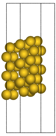
Example

To setup a Au(211) surface with 9 layers and 10 Å of vacuum:

s1 = surface('Au', (2, 1, 1), 9)
s1.center(vacuum=10, axis=2)

This is the easy way, where you use the experimental lattice constant for gold bulk structure. You can write:

from ase.visualize import view
view(s1)

or simply s1.edit() if you want to see and rotate the structure.

Next example is a molybdenum bcc(321) surface where we decide what lattice constant to use:

Mobulk = bulk('Mo', 'bcc', a=3.16, cubic=True)
s2 = surface(Mobulk, (3, 2, 1), 9)
s2.center(vacuum=10, axis=2)

As the last example, creation of alloy surfaces is also very easily carried out with this module. In this example, two Pt₃Rh fcc(211) surfaces will be created:

a = 4.0
Pt3Rh = Atoms('Pt3Rh',
              scaled_positions=[(0, 0, 0),
                                (0.5, 0.5, 0),
                                (0.5, 0, 0.5),
                                (0, 0.5, 0.5)],
              cell=[a, a, a],
              pbc=True)
s3 = surface(Pt3Rh, (2, 1, 1), 9)
s3.center(vacuum=10, axis=2)

Pt3Rh.set_chemical_symbols('PtRhPt2')
s4 = surface(Pt3Rh, (2, 1, 1), 9)
s4.center(vacuum=10, axis=2)