
Constrained minima hopping (global optimization)#
This is an example of a search for a global optimum geometric configuration using the minima hopping algorithm, along with the Hookean class of constraints. This type of approach is useful in searching for the global optimum position of adsorbates on a surface while enforcing that the adsorbates’ identity is preserved.
The below example looks at finding the optimum configuration of a Cu2 adsorbate on a fixed Pt (110) surface. Although this is not a physically relevant simulation — these elements (Cu, Pt) were chosen only because they work with the EMT calculator – one can imagine replacing the Cu2 adsorbate with CO, for example, to find its optimum binding configuration under the constraint that the CO does not dissociate into separate C and O adsorbates.
This also uses the Hookean constraint in two different ways. In the first, it constrains the Cu atoms to feel a restorative force if their interatomic distance exceeds 2.6 Angstroms; this preserves the dimer character of the Cu2, and if they are near each other they feel no constraint. The second constrains one of the Cu atoms to feel a downward force if its position exceeds a z coordinate of 15 Angstroms. Since the Cu atoms are tied together, we don’t necessarily need to put such a force on both of the Cu atoms. This second constraint prevents the Cu2 adsorbate from flying off the surface, which would lead to it exploring a lot of irrelevant configurational space, such as up in the vacuum or on the bottom of the next periodic slab.
from ase import Atom, Atoms
from ase.build import fcc110
from ase.calculators.emt import EMT
from ase.constraints import FixAtoms, Hookean
from ase.optimize.minimahopping import MinimaHopping

# Make the Pt 110 slab.
atoms = fcc110('Pt', (2, 2, 2), vacuum=7.0)

# Add the Cu2 adsorbate.
adsorbate = Atoms(
    [
        Atom('Cu', atoms[7].position + (0.0, 0.0, 2.5)),
        Atom('Cu', atoms[7].position + (0.0, 0.0, 5.0)),
    ]
)
atoms.extend(adsorbate)

# Constrain the surface to be fixed and a Hookean constraint between
# the adsorbate atoms.
constraints = [
    FixAtoms(indices=[atom.index for atom in atoms if atom.symbol == 'Pt']),
    Hookean(a1=8, a2=9, rt=2.6, k=15.0),
    Hookean(a1=8, a2=(0.0, 0.0, 1.0, -15.0), k=15.0),
]
atoms.set_constraint(constraints)

# Set the calculator.
calc = EMT()
atoms.calc = calc

# Instantiate and run the minima hopping algorithm.
hop = MinimaHopping(atoms, Ediff0=2.5, T0=4000.0)
hop(totalsteps=10)
This script will produce 10 molecular dynamics and 11 optimization files. It will also produce a file called ‘minima.traj’ which contains all of the accepted minima. You can look at the progress of the algorithm in the file hop.log in combination with the trajectory files.
Alternatively, there is a utility to allow you to visualize the progress of the algorithm. You can run this from within the same directory as your algorithm as:
from ase.optimize.minimahopping import MHPlot

mhplot = MHPlot()
mhplot.save_figure('summary.png')
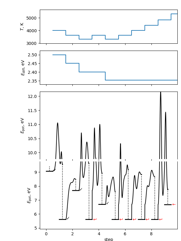
This will make a summary figure, which should look something like the one below. As the search is inherently random, yours will look different than this (and this will look different each time the documentation is rebuilt). In this figure, you will see on the \(E_\mathrm{pot}\) axes the energy levels of the conformers found. The flat bars represent the energy at the end of each local optimization step. The checkmark indicates the local minimum was accepted; red arrows indicate it was rejected for the three possible reasons. The black path between steps is the potential energy during the molecular dynamics (MD) portion of the step; the dashed line is the local optimization on termination of the MD step. Note the y axis is broken to allow different energy scales between the local minima and the space explored in the MD simulations. The \(T\) and \(E_\mathrm{diff}\) plots show the values of the self-adjusting parameters as the algorithm progresses.
You can see examples of the implementation of this for real adsorbates as well as find suitable parameters for the Hookean constraints:
Andrew PetersonTop. Catal., Vol. 57, 40 (2014)