
VASP#
Introduction#
VASP is a density-functional theory code using pseudopotentials or the projector-augmented wave method and a plane wave basis set. This interface makes it possible to use VASP as a calculator in ASE, and also to use ASE as a post-processor for an already performed VASP calculation.
Environment variables#
VASP execution#
You need to add an environment variable which contains instructions
on how to execute VASP. This must be stored as either ASE_VASP_COMMAND
or VASP_COMMAND (the latter for legacy reasons). This could look
something like this:
$ export ASE_VASP_COMMAND="mpirun vasp_std"
This is not required, if the command keyword is specified in the
calculator itself. The command keyword also overrides the enrivonment
variables, e.g.:
Vasp(command='mpiexec vasp_std')
Alternatively, you can write a script called run_vasp.py containing
something like this:
import os
exitcode = os.system('vasp')
The environment variable VASP_SCRIPT must point to that file.
This approach allows for doing other things pre- and post-calculation.
Pseudopotentials#
A directory containing the pseudopotential directories potpaw
(LDA XC) potpaw_GGA (PW91 XC) and potpaw_PBE (PBE XC)
is also needed, and it is to be put in the environment variable
VASP_PP_PATH.
Set both environment variables in your shell configuration file:
$ export VASP_SCRIPT=$HOME/vasp/run_vasp.py
$ export VASP_PP_PATH=$HOME/vasp/mypps
The following environment variable can be used to automatically copy the
van der Waals kernel to the calculation directory. The kernel is needed for
vdW calculations, see VASP vdW wiki, for more details. The kernel is looked
for whenever luse_vdw=True.
$ export ASE_VASP_VDW=$HOME/<path-to-vdw_kernel.bindat-folder>
The environment variable ASE_VASP_VDW should point to the folder where
the vdw_kernel.bindat file is located.
VASP Calculator#
The default setting used by the VASP interface is
- class ase.calculators.vasp.Vasp(atoms=None, restart=None, directory='.', label='vasp', ignore_bad_restart_file=<object object>, command=None, txt='vasp.out', **kwargs)[source]#
ASE interface for the Vienna Ab initio Simulation Package (VASP), with the Calculator interface.
Parameters:
- atoms: object
Attach an atoms object to the calculator.
- label: str
Prefix for the output file, and sets the working directory. Default is ‘vasp’.
- directory: str
Set the working directory. Is prepended to
label.- restart: str or bool
Sets a label for the directory to load files from. if
restart=True, the working directory fromdirectoryis used.- txt: bool, None, str or writable object
If txt is None, output stream will be supressed
If txt is ‘-’ the output will be sent through stdout
If txt is a string a file will be opened, and the output will be sent to that file.
Finally, txt can also be a an output stream, which has a ‘write’ attribute.
Default is ‘vasp.out’
- Examples:
>>> from ase.calculators.vasp import Vasp
>>> calc = Vasp(label='mylabel', txt='vasp.out') # Redirect stdout
>>> calc = Vasp(txt='myfile.txt') # Redirect stdout
>>> calc = Vasp(txt='-') # Print vasp output to stdout
>>> calc = Vasp(txt=None)  # Suppress txt output
- command: str
Custom instructions on how to execute VASP. Has priority over environment variables.
Deprecated since version 3.19.2: Specifying directory in
labelis deprecated, usedirectoryinstead.
Below follows a list with a selection of parameters
keyword |
type |
default value |
description |
|---|---|---|---|
|
|
|
Directory of the VASP run. Defaults to running in the current working directory. |
|
|
None |
Instructions on how to execute VASP.
If this is |
|
Various |
|
Where to redict the stdout text
from the VASP execution.
Defaults to |
|
|
None |
Restart old calculation or use ASE for post-processing |
|
|
‘PW91’ |
XC-functional. Defaults to
None if |
|
|
None |
Additional setup option |
|
|
Set by |
Pseudopotential (POTCAR) set used (LDA, PW91 or PBE). |
|
various |
\(\Gamma\)-point |
k-point sampling |
|
|
None |
\(\Gamma\)-point centered k-point sampling |
|
|
None |
Use reciprocal units if k-points are specified explicitly |
|
|
None |
Net charge per unit cell given in
units of the elementary charge, as
an alternative to specifying
|
|
|
Accuracy of calculation |
|
|
|
Kinetic energy cutoff |
|
|
|
Convergence break condition for SC-loop. |
|
|
|
Number of bands |
|
|
|
Electronic minimization algorithm |
|
|
|
Type of smearing |
|
|
|
Width of smearing |
|
|
|
Maximum number of SC-iterations |
|
|
|
LD(S)A+U parameters |
For parameters in the list without default value given, VASP will set
the default value. Most of the parameters used in the VASP INCAR file
are allowed keywords. See the official VASP manual for more details.
Input arguments specific to the VTST add-ons for VASP are also supported.
Note
Parameters can be changed after the calculator has been constructed
by using the set() method:
>>> calc.set(prec='Accurate', ediff=1E-5)
This would set the precision to Accurate and the break condition
for the electronic SC-loop to 1E-5 eV.
Exchange-correlation functionals#
The xc parameter is used to define a “recipe” of other parameters
including the pseudopotential set pp. It is possible to override
any parameters set with xc by setting them explicitly. For
example, the screening parameter of a HSE calculation might be
modified with
>>> calc = ase.calculators.vasp.Vasp(xc='hse06', hfscreen=0.4)
The default pseudopotential set is potpaw_PBE unless xc or pp
is set to pw91 or lda.
|
Parameters set |
|---|---|
lda, pbe, pw91 |
|
pbesol, revpbe, rpbe, am05 |
|
blyp |
|
tpss, revtpss, m06l |
|
vdw-df, optpbe-vdw |
|
optb88-vdw, obptb86b-vdw |
|
beef-vdw |
|
vdw-df2 |
|
hf |
|
pbe0 |
|
b3lyp |
|
hse03, hse06, hsesol |
|
Additional xc recipes are available for several of the recent functionals from the Truhlar group (i.e. sogga, soga11, n12, n12-sx, mn12l, gam, hle17, revm06l, m06sx), which require VASP to be patched with the MN-VFM module.
It is possible for the user to temporarily add their own xc
recipes without modifying ASE, by updating a dictionary. For example,
to implement a hybrid PW91 calculation:
from ase.calculators.vasp import Vasp
Vasp.xc_defaults['pw91_0'] = {'gga': '91', 'lhfcalc': True}

calc = Vasp(xc='PW91_0')
Note that the dictionary keys must be lower case, while the xc
parameter is case-insensitive when used.
Setups#
For many elements, VASP is distributed with a choice of pseudopotential setups. These may be hard/soft variants of the pseudopotential or include additional valence electrons. Three base setups are provided:
- minimal (default):
If a PAW folder exists with the same name as the element, this will be used. For the other elements, the PAW setup with the least electrons has been chosen.
- recommended:
corresponds to the table of recommended PAW setups supplied by the VASP developers.
- gw:
corresponds to the table of recommended setups for GW supplied by the VASP developers.
Where elements are missing from the default sets, the Vasp Calculator
will attempt to use a setup folder with the same name as the element.
A default setup may be selected with the setups keyword:
from ase.calculators.vasp import Vasp
calc = Vasp(setups='recommended')
To use an alternative setup for all instances of an element, use the
dictionary form of setups to provide the characters which need
to be added to the element name, e.g.
calc = Vasp(xc='PBE', setups={'Li': '_sv'})
will use the Li_sv all-electron pseudopotential for all Li atoms.
To apply special setups to individual atoms, identify them by their zero-indexed number in the atom list and use the full setup name. For example,
calc = Vasp(xc='PBE', setups={3: 'Ga_d'})
will treat the Ga atom in position 3 (i.e. the fourth atom) of the
atoms object as special, with an additional 10 d-block valence
electrons, while other Ga atoms use the default 3-electron setup and
other elements use their own default setups. The positional index may
be quoted as a string (e.g. {'3': 'Ga_d'}).
These approaches may be combined by using the ‘base’ key to access a default set, e.g.
calc = Vasp(xc='PBE', setups={'base': 'recommended', 'Li': '', 4: 'H.5'})
Spin-polarized calculation#
If the atoms object has non-zero magnetic moments, a spin-polarized calculation will be performed by default.
Here follows an example how to calculate the total magnetic moment of a sodium chloride molecule.
from ase import Atom, Atoms
from ase.calculators.vasp import Vasp

a = [6.5, 6.5, 7.7]
d = 2.3608
NaCl = Atoms(
    [Atom('Na', [0, 0, 0], magmom=1.928), Atom('Cl', [0, 0, d], magmom=0.75)],
    cell=a,
)

calc = Vasp(prec='Accurate', xc='PBE', lreal=False)
NaCl.calc = calc

print(NaCl.get_magnetic_moment())
In this example the initial magnetic moments are assigned to the atoms
when defining the Atoms object. The calculator will detect that at least
one of the atoms has a non-zero magnetic moment and a spin-polarized
calculation will automatically be performed. The ASE generated INCAR
file will look like:
INCAR created by Atomic Simulation Environment
 PREC = Accurate
 LREAL = .FALSE.
 ISPIN = 2
 MAGMOM = 1*1.9280 1*0.7500
Note
It is also possible to manually tell the calculator to perform a spin-polarized calculation:
>>> calc.set(ispin=2)
This can be useful for continuation jobs, where the initial magnetic moment is read from the WAVECAR file.
Brillouin-zone sampling#
Brillouin-zone sampling is controlled by the parameters kpts,
gamma and reciprocal, and may also be set with the VASP
parameters kspacing and kgamma.
Single-parameter schemes#
A k-point mesh may be set using a single value in one of two ways:
- Scalar
kpts If
kptsis declared as a scalar (i.e. a float or an int), an appropriate KPOINTS file will be written. The value ofkptswill be used to set a length cutoff for the Gamma-centered “Automatic” scheme provided by VASP. (See first example in VASP manual.)- KSPACING and KGAMMA
Alternatively, the k-point density can be set in the INCAR file with these flags as described in the VASP manual. If
kspacingis set, the ASE calculator will not write out a KPOINTS file.
Three-parameter scheme#
Brillouin-zone sampling can also be specified by defining a number of subdivisions for each reciprocal lattice vector.
This is the second “Automatic” scheme described in the VASP manual.
In the ASE calculator, it is used by setting kpts to a sequence of three int values, e.g. [2, 2, 3].
If gamma` is set to ``True, the mesh will be centred at the \(\Gamma\)-point;
otherwise, a regular Monkhorst-Pack grid is used, which may or may not include the \(\Gamma\)-point.
In VASP it is possible to define an automatic grid and shift the origin point.
This function is not currently included in the ASE calculator. The same result can be achieved by using ase.dft.kpoints.monkhorst_pack() to generate an explicit list of k-points (see below) and simply adding a constant vector to the matrix.
For example,
import ase.dft.kpoints
kpts = ase.dft.kpoints.monkhorst_pack([2, 2, 1]) + [0.25, 0.25, 0.5]
creates an acceptable kpts array with the values
array([[ 0. ,  0. ,  0.5],
       [ 0. ,  0.5,  0.5],
       [ 0.5,  0. ,  0.5],
       [ 0.5,  0.5,  0.5]])
However, this method will prevent VASP from using symmetry to reduce the number of calculated points.
Explicitly listing the k-points#
If an n-by-3 or n-by-4 array is used for kpts,
this is interpreted as a list of n explicit k-points and an appropriate KPOINTS file is generated.
The fourth column, if provided, sets the sample weighting of each point.
Otherwise, all points are weighted equally.
Usually in these cases it is desirable to set the reciprocal parameter to True,
so that the k-point vectors are given relative to the reciprocal lattice.
Otherwise, they are taken as being in Cartesian space.
Band structure paths#
VASP provides a “line-mode” for the generation of band-structure paths.
While this is not directly supported by ASE, relevant functionality exists in the ase.dft.kpoints module.
For example:
import ase.build
from ase.dft.kpoints import bandpath

si = ase.build.bulk('Si')
kpts, x_coords, x_special_points = bandpath('GXL', si.cell, npoints=20)
returns an acceptable kpts array (for use with reciprocal=True) as well as plotting information.
LD(S)A+U#
The VASP +U corrections can be turned on using the default VASP parameters explicitly, by manually setting
the ldaul, ldauu and ldauj parameters, as well as enabling ldau.
However, ASE offers a convenient ASE specific keyword to enable these, by using a dictionary construction, through the
ldau_luj keyword. If the user does not explicitly set ldau=False, then ldau=True will automatically
be set if ldau_luj is set.
For example:
calc = Vasp(ldau_luj={'Si': {'L': 1, 'U': 3, 'J': 0}})
will set U=3 on the Si p-orbitals, and will automatically set ldau=True as well.
Restart old calculation#
To continue an old calculation which has been performed without the interface
use the restart parameter when constructing the calculator
>>> calc = Vasp(restart=True)
Then the calculator will read atomic positions from the CONTCAR file,
physical quantities from the OUTCAR file, k-points from the
KPOINTS file and parameters from the INCAR file.
Note
Only Monkhorst-Pack and Gamma-centered k-point sampling are supported
for restart at the moment. Some INCAR parameters may not be
implemented for restart yet. Please report any problems to the ASE mailing
list.
The restart parameter can be used , as the name suggest to continue a job from where a
previous calculation finished. Furthermore, it can be used to extract data from
an already performed calculation. For example, to get the total potential energy
of the sodium chloride molecule in the previous section, without performing any additional
calculations, in the directory of the previous calculation do:
>>> calc = Vasp(restart=True)
>>> atoms = calc.get_atoms()
>>> atoms.get_potential_energy()
-4.7386889999999999
Storing the calculator state#
The results from the Vasp calculator can exported as a dictionary, which can then be saved in a JSON format,
which enables easy and compressed sharing and storing of the input & outputs of
a VASP calculation. The following methods of Vasp can be used for this purpose:
- Vasp.asdict()[source]#
Return a dictionary representation of the calculator state. Does NOT contain information on the
command,txtordirectorykeywords. Contains the following keys:ase_versionvasp_versioninputsresultsatoms(Only if the calculator has anAtomsobject)
- Vasp.fromdict(dct)[source]#
Restore calculator from a
asdict()dictionary.Parameters:
- dct: Dictionary
The dictionary which is used to restore the calculator state.
- Vasp.write_json(filename)[source]#
Dump calculator state to JSON file.
Parameters:
- filename: string
The filename which the JSON file will be stored to. Prepends the
directorypath to the filename.
First we can dump the state of the calculation using the write_json() method:
# After a calculation
calc.write_json('mystate.json')

# This is equivalent to
from ase.io import jsonio
dct = calc.asdict()  # Get the calculator in a dictionary format
jsonio.write_json('mystate.json', dct)
At a later stage, that file can be used to restore a the input and (simple) output parameters of a calculation,
without the need to copy around all the VASP specific files, using either the ase.io.jsonio.read_json() function
or the Vasp fromdict() method.
calc = Vasp()
calc.read_json('mystate.json')
atoms = calc.get_atoms()  # Get the atoms object

# This is equivalent to
from ase.calculators.vasp import Vasp
from ase.io import jsonio
dct = jsonio.read_json('mystate.json')  # Load exported dict object from the JSON file
calc = Vasp()
calc.fromdict(dct)
atoms = calc.get_atoms()  # Get the atoms object
The dictionary object, which is created from the todict() method, also contains information about the ASE
and VASP version which was used at the time of the calculation, through the
ase_version and vasp_version keys.
import json
with open('mystate.json', 'r') as f:
    dct = json.load(f)
print('ASE version: {}, VASP version: {}'.format(dct['ase_version'], dct['vasp_version']))
Note
The ASE calculator contains no information about the wavefunctions or charge densities, so these are NOT stored in the dictionary or JSON file, and therefore results may vary on a restarted calculation.
Vibrational Analysis#
Vibrational analysis can be performed using the Vibrations
class or using the VASP internals (e.g. with IBRION=5).
When using IBRION=5-8, the corresponding vibrational
analysis can be represented by retrieving a VibrationsData
object from the calculator using ase.calculators.vasp.Vasp.get_vibrations().
From the OUTCAR, the energies of all modes can be retrieved using
ase.calculators.vasp.Vasp.read_vib_freq().
- Vasp.get_vibrations() VibrationsData[source]#
Get a VibrationsData Object from a VASP Calculation.
- Returns:
VibrationsData object.
Note that the atoms in the VibrationsData object can be resorted.
Uses the (mass weighted) Hessian from vasprun.xml, different masses in the POTCAR can therefore result in different results.
Note the limitations concerning k-points and symmetry mentioned in the VASP-Wiki.
Examples#
The Vasp 2 calculator now integrates with existing ASE functions, such as
BandStructure or bandgap.
Band structure with VASP#
The VASP manual has an example of creating a Si band structure - we can easily reproduce a similar result, by using the ASE Vasp calculator.
We can use the directory keyword to control the folder in which the calculations
take place, and keep a more structured folder structure. The following script does the
initial calculations, in order to construct the band structure for silicon
from ase.build import bulk
from ase.calculators.vasp import Vasp

si = bulk('Si')

mydir = 'bandstructure'    # Directory where we will do the calculations

# Make self-consistent ground state
calc = Vasp(kpts=(4, 4, 4), directory=mydir)

si.calc = calc
si.get_potential_energy()  # Run the calculation

# Non-SC calculation along band path
kpts = {'path': 'WGX',     # The BS path
        'npoints': 30}     # Number of points along the path

calc.set(isym=0,           # Turn off kpoint symmetry reduction
         icharg=11,        # Non-SC calculation
         kpts=kpts)

# Run the calculation
si.get_potential_energy()
As this calculation might be longer, depending on your system, it may
be more convenient to split the plotting into a separate file, as all
of the VASP data is written to files. The plotting can then be achieved
by using the restart keyword, in a second script
from ase.calculators.vasp import Vasp

mydir = 'bandstructure'    # Directory where we did the calculations

# Load the calculator from the VASP output files
calc_load = Vasp(restart=True, directory=mydir)

bs = calc_load.band_structure() # ASE Band structure object
bs.plot(emin=-13, show=True)    # Plot the band structure
Which results in the following image
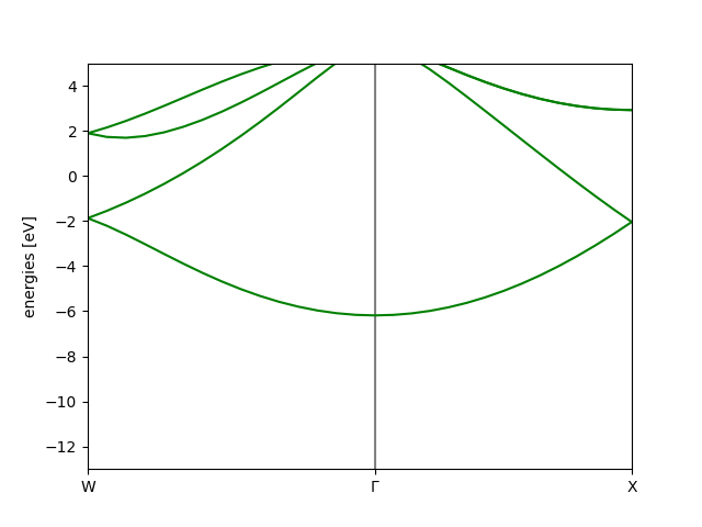
We could also find the band gap in the same calculation,
>>> from ase.dft.bandgap import bandgap
>>> bandgap(calc_load)
Gap: 0.474 eV
Transition (v -> c):
  (s=0, k=15, n=3, [0.000, 0.000, 0.000]) -> (s=0, k=27, n=4, [0.429, 0.000, 0.429])
Note
When using hybrids, due to the exact-exchange calculations, one needs to treat the k-point sampling more carefully, see VASP HSE band structure wiki.
Currently, we have no functions to easily handle this issue, but may be added in the future.
Density of States#
The Vasp calculator also allows for quick access to the Density of States (DOS), through the ASE DOS module, see DOS.
Quick access to this function, however, can be found by using the get_dos() function:
>>> energies, dos = calc.get_dos()