Brillouin zone sampling¶

The k-points are always given relative to the basis vectors of the reciprocal unit cell.

Monkhorst-Pack¶

ase.dft.kpoints.monkhorst_pack(size)[source]¶: Construct a uniform sampling of k-space of given size.

The k-points are given as [MonkhorstPack]:

\[\sum_{i=1,2,3} \frac{2n_i -N_i - 1}{2N_i} \mathbf{b}_i,\]

where \(n_i=1,2,...,N_i\), size = \((N_1, N_2, N_3)\) and the \(\mathbf{b}_i\)’s are reciprocal lattice vectors.

ase.dft.kpoints.get_monkhorst_pack_size_and_offset(kpts)[source]¶

Find Monkhorst-Pack size and offset.

Returns (size, offset), where:

kpts = monkhorst_pack(size) + offset.

The set of k-points must not have been symmetry reduced.

Example:

>>> from ase.dft.kpoints import *
>>> monkhorst_pack((4, 1, 1))
array([[-0.375,  0.   ,  0.   ],
       [-0.125,  0.   ,  0.   ],
       [ 0.125,  0.   ,  0.   ],
       [ 0.375,  0.   ,  0.   ]])
>>> get_monkhorst_pack_size_and_offset([[0, 0, 0]])
(array([1, 1, 1]), array([ 0.,  0.,  0.]))

[MonkhorstPack]

Hendrik J. Monkhorst and James D. Pack: Special points for Brillouin-zone integrations, Phys. Rev. B 13, 5188–5192 (1976) doi: 10.1103/PhysRevB.13.5188

Special points in the Brillouin zone¶

ase.dft.kpoints.special_points¶

The below table lists the special points from [Setyawan-Curtarolo].

Brillouin zone data

Brillouin zone data¶

CUB (primitive cubic)	GXMGRX,MR
FCC (face-centred cubic)	GXWKGLUWLK,UX
BCC (body-centred cubic)	GHNGPH,PN
TET (primitive tetragonal)	GXMGZRAZ,XR,MA
BCT1 (body-centred tetragonal)	GXMGZPNZ1M,XP
BCT2 (body-centred tetragonal)	GXYSGZS1NPY1Z,XP
ORC (primitive orthorhombic)	GXSYGZURTZ,YT,UX,SR
ORCF1 (face-centred orthorhombic)	GYTZGXA1Y,TX1,XAZ,LG
ORCF2 (face-centred orthorhombic)	GYCDXGZD1HC,C1Z,XH1,HY,LG
ORCF3 (face-centred orthorhombic)	GYTZGXA1Y,XAZ,LG
ORCI (body-centred orthorhombic)	GXLTWRX1ZGYSW,L1Y,Y1Z
ORCC (base-centred orthorhombic)	GXSRAZGYX1A1TY,ZT
HEX (primitive hexagonal)	GMKGALHA,LM,KH
RHL1 (primitive rhombohedral)	GLB1,BZGX,QFP1Z,LP
RHL2 (primitive rhombohedral)	GPZQGFP1Q1LZ
MCL (primitive monoclinic)	GYHCEM1AXH1,MDZ,YD
MCLC1 (base-centred monoclinic)	GYFLI,I1ZF1,YX1,XGN,MG
MCLC3 (base-centred monoclinic)	GYFHZIF1,H1Y1XGN,MG
MCLC5 (base-centred monoclinic)	GYFLI,I1ZHF1,H1Y1XGN,MG
TRI1a (primitive triclinic)	XGY,LGZ,NGM,RG
TRI1b (primitive triclinic)	XGY,LGZ,NGM,RG
TRI2a (primitive triclinic)	XGY,LGZ,NGM,RG
TRI2b (primitive triclinic)	XGY,LGZ,NGM,RG
OBL (primitive oblique)	GYHCH1XG
RECT (primitive rectangular)	GXSYGS
CRECT (centred rectangular)	GXA1YG
HEX2D (primitive hexagonal)	GMKG
SQR (primitive square)	MGXM
LINE (primitive line)	GX

[Setyawan-Curtarolo] (1,2)

High-throughput electronic band structure calculations: Challenges and tools

Wahyu Setyawan, Stefano Curtarolo

Computational Materials Science, Volume 49, Issue 2, August 2010, Pages 299–312

doi: 10.1016/j.commatsci.2010.05.010

You can find the special points in the Brillouin zone:

>>> from ase.build import bulk
>>> si = bulk('Si', 'diamond', a=5.459)
>>> lat = si.cell.get_bravais_lattice()
>>> print(list(lat.get_special_points()))
['G', 'K', 'L', 'U', 'W', 'X']
>>> path = si.cell.bandpath('GXW', npoints=100)
>>> print(path.kpts.shape)
(100, 3)

ase.dft.kpoints.get_special_points(cell, lattice=None, eps=0.0002)[source]¶

Return dict of special points.

The definitions are from a paper by Wahyu Setyawana and Stefano Curtarolo:

https://doi.org/10.1016/j.commatsci.2010.05.010

cell: 3x3 ndarray: Unit cell.
lattice: str: Optionally check that the cell is one of the following: cubic, fcc, bcc, orthorhombic, tetragonal, hexagonal or monoclinic.
eps: float: Tolerance for cell-check.

ase.dft.kpoints.bandpath(path, cell, npoints=None, density=None, special_points=None, eps=0.0002)[source]¶

Make a list of kpoints defining the path between the given points.

path: list or str

Can be:

a string that parse_path_string() understands: ‘GXL’
a list of BZ points: [(0, 0, 0), (0.5, 0, 0)]
or several lists of BZ points if the the path is not continuous.

cell: 3x3

Unit cell of the atoms.

npoints: int

Length of the output kpts list. If too small, at least the beginning and ending point of each path segment will be used. If None (default), it will be calculated using the supplied density or a default one.

density: float

k-points per 1/A on the output kpts list. If npoints is None, the number of k-points in the output list will be: npoints = density * path total length (in Angstroms). If density is None (default), use 5 k-points per A⁻¹. If the calculated npoints value is less than 50, a minimum value of 50 will be used.

special_points: dict or None

Dictionary mapping names to special points. If None, the special points will be derived from the cell.

eps: float

Precision used to identify Bravais lattice, deducing special points.

You may define npoints or density but not both.

Return a BandPath object.

ase.dft.kpoints.parse_path_string(s)[source]¶

Parse compact string representation of BZ path.

A path string can have several non-connected sections separated by commas. The return value is a list of sections where each section is a list of labels.

Examples:

>>> parse_path_string('GX')
[['G', 'X']]
>>> parse_path_string('GX,M1A')
[['G', 'X'], ['M1', 'A']]

ase.dft.kpoints.labels_from_kpts(kpts, cell, eps=1e-05, special_points=None)[source]¶

Get an x-axis to be used when plotting a band structure.

The first of the returned lists can be used as a x-axis when plotting the band structure. The second list can be used as xticks, and the third as xticklabels.

Parameters:

kpts: list: List of scaled k-points.
cell: list: Unit cell of the atomic structure.

Returns:

Three arrays; the first is a list of cumulative distances between k-points, the second is x coordinates of the special points, the third is the special points as strings.

Band path¶

The BandPath class stores all the relevant band path information in a single object. It is typically created by helper functions such as ase.cell.Cell.bandpath() or ase.lattice.BravaisLattice.bandpath().

class ase.dft.kpoints.BandPath(cell, kpts=None, special_points=None, path=None)[source]¶

Represents a Brillouin zone path or bandpath.

A band path has a unit cell, a path specification, special points, and interpolated k-points. Band paths are typically created indirectly using the Cell or BravaisLattice classes:

>>> from ase.lattice import CUB
>>> path = CUB(3).bandpath()
>>> path
BandPath(path='GXMGRX,MR', cell=[3x3], special_points={GMRX}, kpts=[40x3])

Band paths support JSON I/O:

>>> from ase.io.jsonio import read_json
>>> path.write('mybandpath.json')
>>> read_json('mybandpath.json')
BandPath(path='GXMGRX,MR', cell=[3x3], special_points={GMRX}, kpts=[40x3])

cartesian_kpts() → ndarray[source]¶: Get Cartesian kpoints from this bandpath.

property cell: Cell¶: The Cell of this BandPath.

free_electron_band_structure(**kwargs) → BandStructure[source]¶

Return band structure of free electrons for this bandpath.

Keyword arguments are passed to FreeElectrons.

This is for mostly testing and visualization.

get_linear_kpoint_axis(eps=1e-05)[source]¶

Define x axis suitable for plotting a band structure.

See ase.dft.kpoints.labels_from_kpts().

property icell: Cell¶: Reciprocal cell of this BandPath as a Cell.

interpolate(path: str = None, npoints: int = None, special_points: Dict[str, ndarray] = None, density: float = None) → BandPath[source]¶: Create new bandpath, (re-)interpolating kpoints from this one.

property kpts: ndarray¶

The kpoints of this BandPath as an array of shape (nkpts, 3).

The kpoints are given in units of the reciprocal cell.

property path: str¶

The string specification of this band path.

This is a specification of the form \('GXWKGLUWLK,UX'\).

Comma marks a discontinuous jump: K is not connected to U.

plot(**plotkwargs)[source]¶

Visualize this bandpath.

Plots the irreducible Brillouin zone and this bandpath.

classmethod read(fd)¶: Read new instance from JSON file.

property special_points: Dict[str, ndarray]¶

Special points of this BandPath as a dictionary.

The dictionary maps names (such as \('G'\)) to kpoint coordinates in units of the reciprocal cell as a 3-element numpy array.

It’s unwise to edit this dictionary directly. If you need that, consider deepcopying it.

transform(op: ndarray) → BandPath[source]¶

Apply 3x3 matrix to this BandPath and return new BandPath.

This is useful for converting the band path to another cell. The operation will typically be a permutation/flipping established by a function such as Niggli reduction.

write(fd)¶: Write to JSON file.

Band structure¶

class ase.spectrum.band_structure.BandStructure(path, energies, reference=0.0)[source]¶

A band structure consists of an array of eigenvalues and a bandpath.

BandStructure objects support JSON I/O.

property energies: ndarray¶

The energies of this band structure.

This is a numpy array of shape (nspins, nkpoints, nbands).

get_labels(eps=1e-05)[source]¶: “See ase.dft.kpoints.labels_from_kpts().

property path: BandPath¶: The BandPath of this band structure.

plot(*args, **kwargs)[source]¶: Plot this band structure.

classmethod read(fd)¶: Read new instance from JSON file.

property reference: float¶

The reference energy.

Semantics may vary; typically a Fermi energy or zero, depending on how the band structure was created.

subtract_reference() → BandStructure[source]¶: Return new band structure with reference energy subtracted.

write(fd)¶: Write to JSON file.

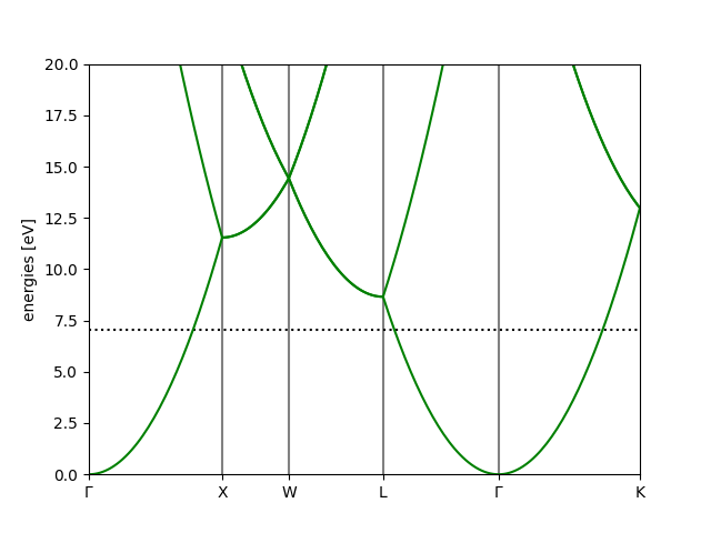
Free electron example:

# creates: cu.png
from ase.build import bulk
from ase.calculators.test import FreeElectrons

a = bulk('Cu')
a.calc = FreeElectrons(nvalence=1,
                       kpts={'path': 'GXWLGK', 'npoints': 200})
a.get_potential_energy()
bs = a.calc.band_structure()
bs.plot(emin=0, emax=20, filename='cu.png')

Interpolation¶

ase.dft.kpoints.monkhorst_pack_interpolate(path, values, icell, bz2ibz, size, offset=(0, 0, 0), pad_width=2)[source]¶

Interpolate values from Monkhorst-Pack sampling.

\(monkhorst_pack_interpolate\) takes a set of \(values\), for example eigenvalues, that are resolved on a Monkhorst Pack k-point grid given by \(size\) and \(offset\) and interpolates the values onto the k-points in \(path\).

Note

For the interpolation to work, path has to lie inside the domain that is spanned by the MP kpoint grid given by size and offset.

To try to ensure this we expand the domain slightly by adding additional entries along the edges and sides of the domain with values determined by wrapping the values to the opposite side of the domain. In this way we assume that the function to be interpolated is a periodic function in k-space. The padding width is determined by the \(pad_width\) parameter.

Parameters:

path ((nk, 3) array-like) – Desired path in units of reciprocal lattice vectors.
values ((nibz, ...) array-like) – Values on Monkhorst-Pack grid.
icell ((3, 3) array-like) – Reciprocal lattice vectors.
bz2ibz ((nbz,) array-like of int) – Map from nbz points in BZ to nibz reduced points in IBZ.
size ((3,) array-like of int) – Size of Monkhorst-Pack grid.
offset ((3,) array-like) – Offset of Monkhorst-Pack grid.
pad_width (int) – Padding width to aid interpolation

Returns:

values interpolated to path.

Return type:

(nbz,) array-like

High symmetry paths¶

ase.dft.kpoints.special_paths¶

The ase.lattice framework provides suggestions for high symmetry paths in the BZ from the [Setyawan-Curtarolo] paper.

>>> from ase.lattice import BCC
>>> lat = BCC(3.5)
>>> lat.get_special_points()
{'G': array([0, 0, 0]), 'H': array([ 0.5, -0.5,  0.5]), 'P': array([0.25, 0.25, 0.25]), 'N': array([0. , 0. , 0.5])}
>>> lat.special_path
'GHNGPH,PN'

In case you want this information without providing the lattice parameter (which is possible for those lattices where the points do not depend on the lattice parameters), the data is also available as dictionaries:

>>> from ase.dft.kpoints(import special_paths, sc_special_points,
...                      parse_path_string)
>>> paths = sc_special_paths['bcc']
>>> paths
[['G', 'H', 'N', 'G', 'P', 'H'], ['P', 'N']]
>>> points = sc_special_points['bcc']
>>> points
{'H': [0.5, -0.5, 0.5], 'N': [0, 0, 0.5], 'P': [0.25, 0.25, 0.25],
 'G': [0, 0, 0]}
>>> kpts = [points[k] for k in paths[0]]  # G-H-N-G-P-H
>>> kpts
[[0, 0, 0], [0.5, -0.5, 0.5], [0, 0, 0.5], [0, 0, 0], [0.25, 0.25, 0.25], [0.5, -0.5, 0.5]]

Chadi-Cohen¶

Predefined sets of k-points:

ase.dft.kpoints.cc6_1x1¶

ase.dft.kpoints.cc12_2x3¶

ase.dft.kpoints.cc18_sq3xsq3¶

ase.dft.kpoints.cc18_1x1¶

ase.dft.kpoints.cc54_sq3xsq3¶

ase.dft.kpoints.cc54_1x1¶

ase.dft.kpoints.cc162_sq3xsq3¶

ase.dft.kpoints.cc162_1x1¶

Naming convention: cc18_sq3xsq3 is 18 k-points for a sq(3)xsq(3) cell.

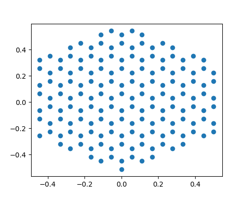
Try this:

>>> import numpy as np
>>> import matplotlib.pyplot as plt
>>> from ase.dft.kpoints import cc162_1x1
>>> B = [(1, 0, 0), (-0.5, 3**0.5 / 2, 0), (0, 0, 1)]
>>> k = np.dot(cc162_1x1, B)
>>> plt.plot(k[:, 0], k[:, 1], 'o')  
[<matplotlib.lines.Line2D object at 0x9b61dcc>]
>>> plt.show()