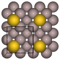
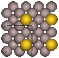
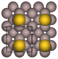
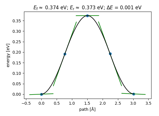
Surface diffusion energy barriers using the Nudged Elastic Band (NEB) method

First, set up the initial and final states:

from ase.build import add_adsorbate, fcc100
from ase.calculators.emt import EMT
from ase.constraints import FixAtoms
from ase.optimize import QuasiNewton

# 2x2-Al(001) surface with 3 layers and an
# Au atom adsorbed in a hollow site:
slab = fcc100('Al', size=(2, 2, 3))
add_adsorbate(slab, 'Au', 1.7, 'hollow')
slab.center(axis=2, vacuum=4.0)

# Make sure the structure is correct:
# view(slab)

# Fix second and third layers:
mask = [atom.tag > 1 for atom in slab]
# print(mask)
slab.set_constraint(FixAtoms(mask=mask))

# Use EMT potential:
slab.calc = EMT()

# Initial state:
qn = QuasiNewton(slab, trajectory='initial.traj')
qn.run(fmax=0.05)

# Final state:
slab[-1].x += slab.get_cell()[0, 0] / 2
qn = QuasiNewton(slab, trajectory='final.traj')
qn.run(fmax=0.05)

Note

Notice how the tags are used to select the constrained atoms

Now, do the NEB calculation:

from ase.calculators.emt import EMT
from ase.constraints import FixAtoms
from ase.io import read
from ase.mep import NEB
from ase.optimize import BFGS

initial = read('initial.traj')
final = read('final.traj')

constraint = FixAtoms(mask=[atom.tag > 1 for atom in initial])

images = [initial]
for i in range(3):
    image = initial.copy()
    image.calc = EMT()
    image.set_constraint(constraint)
    images.append(image)

images.append(final)

neb = NEB(images)
neb.interpolate()
qn = BFGS(neb, trajectory='neb.traj')
qn.run(fmax=0.05)

Visualize the results with:

$ ase gui neb.traj@-5:

and select Tools->NEB.

You can also create a series of plots like above, that show the progression of the NEB relaxation, directly at the command line:

$ ase nebplot --share-x --share-y neb.traj

For more customizable analysis of the output of many NEB jobs, you can use the ase.mep.NEBTools class. Some examples of its use are below; the final example was used to make the figure you see above.

import matplotlib.pyplot as plt

from ase.io import read
from ase.mep import NEBTools

images = read('neb.traj@-5:')

nebtools = NEBTools(images)

# Get the calculated barrier and the energy change of the reaction.
Ef, dE = nebtools.get_barrier()

# Get the barrier without any interpolation between highest images.
Ef, dE = nebtools.get_barrier(fit=False)

# Get the actual maximum force at this point in the simulation.
max_force = nebtools.get_fmax()

# Create a figure like that coming from ASE-GUI.
fig = nebtools.plot_band()
fig.savefig('diffusion-barrier.png')

# Create a figure with custom parameters.
fig = plt.figure(figsize=(5.5, 4.0))
ax = fig.add_axes((0.15, 0.15, 0.8, 0.75))
nebtools.plot_band(ax)
fig.savefig('diffusion-barrier.png')

Note

For this reaction, the reaction coordinate is very simple: The x-coordinate of the Au atom. In such cases, the NEB method is overkill, and a simple constraint method should be used like in this tutorial: Surface diffusion energy barriers using ASE constraints.

See also

• ase.mep.neb

• ase.constraints

• Surface diffusion energy barriers using ASE constraints

• fcc100()

Restarting NEB

Restart NEB from the trajectory file:

from ase.calculators.emt import EMT
from ase.io import read
from ase.mep import NEB
from ase.optimize import BFGS

# read the last structures (of 5 images used in NEB)
images = read('neb.traj@-5:')

for i in range(1, len(images) - 1):
    images[i].calc = EMT()

neb = NEB(images)
qn = BFGS(neb, trajectory='neb_restart.traj')
qn.run(fmax=0.005)

Parallelizing over images with MPI

Instead of having one process do the calculations for all three internal images in turn, it will be faster to have three processes do one image each. In order to be able to run python with MPI you need a special parallel python interpreter, for example gpaw-python.

The example below can then be run with mpiexec -np 3 gpaw-python diffusion3.py:

from ase.calculators.emt import EMT
from ase.constraints import FixAtoms
from ase.io import read
from ase.mep import NEB
from ase.optimize import BFGS
from ase.parallel import world

initial = read('initial.traj')
final = read('final.traj')

constraint = FixAtoms(mask=[atom.tag > 1 for atom in initial])

images = [initial]
j = world.rank * 3 // world.size  # my image number
for i in range(3):
    image = initial.copy()
    if i == j:
        image.calc = EMT()
    image.set_constraint(constraint)
    images.append(image)
images.append(final)

neb = NEB(images, parallel=True)
neb.interpolate()
qn = BFGS(neb, trajectory='neb.traj')
qn.run(fmax=0.05)