
Determination of convex hull with a genetic algorithm#
In this tutorial we will determine the convex hull of a binary alloy slab. The convex hull can be used to check whether a certain composition is stable or it will decompose into mixed phases of the neighboring stable compositions. We will use a (111) slab to represent a close packed surface, the method can easily be extended for use in other systems, e.g. bulk, nanoparticle, … We choose a rather small atomic structure with 24 atoms in the unit cell, in a binary system the number of different atomic distributions for a single composition is determined by the binomial coefficient \(\frac{N!}{n_A!n_B!}\), where \(N\) is the total number of atoms in the slab, \(n_A\) and \(n_B\) is the number of A and B atoms respectively. This number rises combinatorially towards the 1:1 composition and in total there exists 16.8 million different atomic distributions for the 24 atom slab (without taking symmetry into account which will reduce the number significantly see Symmetric duplicate identification). A number of this size warrants a search method other than brute force, here we use a genetic algorithm (GA).
Outline of the GA run#
The GA implementation is divided into several classes, this means that the user can pick and choose specific classes and functions to use for the optimization problem at hand. If no ready-made crossover operator works for a specific problem it should be quite straightforward to customize an existing one.
We will create an initial population of (111) slabs each with a random composition and distribution of atoms.
The candidates are evaluated with the EMT potential. To make comparisons between different compositions we define the mixing or excess energy by:
where \(E_\text{AB}\) is the energy of the mixed slab, \(E_A\) and \(E_B\) are the energies of the pure A and B slabs respectively.
We will take advantage of the ase.ga.population.RankFitnessPopulation, that allows us to optimize a full composition range at once. It works by grouping candidates according to a variable (composition in this case) and then ranking candidates within each group. This means that the fittest candidate in each group is given equal fitness and has the same probability for being selected for procreation. This means that the entire convex hull is mapped out contrary to just the candidates with lowest mixing energies. This “all in one” approach is more efficient than running each composition individually since the chemical ordering is similar for different compositions.
We will use the typical operators adjusted to work on slabs: CutSpliceSlabCrossover cuts two slabs in a random plane and put halves from different original slabs (parents) together to form a new slab (offspring). This Deaven and Ho style crossover is able to refine the population by passing on favorable traits from parents to offspring. RandomSlabPermutation permutes two atoms of different type in the slab keeping the same composition. RandomCompositionMutation changes the composition of the slab.
In Customization of the algorithm we look at ways to customize the way in which the algorithm runs in order to make it more efficient.
Initial population#
We choose a population size large enough so that the entire composition range will be represented in the population. The pure slabs are set up using experimental lattice constants, and for the mixed slabs we use Vegard’s law (interpolation). ga_convex_start.py
import random
from pathlib import Path

from ase.build import fcc111
from ase.calculators.emt import EMT
from ase.data import atomic_numbers, reference_states
from ase.ga import set_raw_score
from ase.ga.data import PrepareDB


def get_avg_lattice_constant(syms):
    a = 0.0
    for m in set(syms):
        a += syms.count(m) * lattice_constants[m]
    return a / len(syms)


metals = ['Cu', 'Pt']
# Use experimental lattice constants
lattice_constants = {
    m: reference_states[atomic_numbers[m]]['a'] for m in metals
}

# Create the references (pure slabs) manually
pure_slabs = []
refs = {}
print('Reference energies:')
for m in metals:
    slab = fcc111(
        m, size=(2, 4, 3), a=lattice_constants[m], vacuum=5, orthogonal=True
    )
    slab.calc = EMT()

    # We save the reference energy as E_A / N
    e = slab.get_potential_energy()
    e_per_atom = e / len(slab)
    refs[m] = e_per_atom
    print(f'{m} = {e_per_atom:.3f} eV/atom')

    # The mixing energy for the pure slab is 0 by definition
    set_raw_score(slab, 0.0)
    pure_slabs.append(slab)

# The population size should be at least the number of different compositions
pop_size = 2 * len(slab)

# We prepare the db and write a few constants that we are going to use later
target = Path('hull.db')
if target.exists():
    target.unlink()
db = PrepareDB(
    target,
    population_size=pop_size,
    reference_energies=refs,
    metals=metals,
    lattice_constants=lattice_constants,
)

# We add the pure slabs to the database as relaxed because we have already
# set the raw_score
for slab in pure_slabs:
    db.add_relaxed_candidate(
        slab, atoms_string=''.join(slab.get_chemical_symbols())
    )


# Now we create the rest of the candidates for the initial population
for i in range(pop_size - 2):
    # How many of each metal is picked at random, making sure that
    # we do not pick pure slabs
    nA = random.randint(0, len(slab) - 2)
    nB = len(slab) - 2 - nA
    symbols = [metals[0]] * nA + [metals[1]] * nB + metals

    # Making a generic slab with the correct lattice constant
    slab = fcc111(
        'X',
        size=(2, 4, 3),
        a=get_avg_lattice_constant(symbols),
        vacuum=5,
        orthogonal=True,
    )

    # Setting the symbols and randomizing the order
    slab.set_chemical_symbols(symbols)
    random.shuffle(slab.numbers)

    # Add these candidates as unrelaxed, we will relax them later
    atoms_string = ''.join(slab.get_chemical_symbols())
    db.add_unrelaxed_candidate(slab, atoms_string=atoms_string)
Now we have the file hull.db, that can be examined like a regular ase.db database. The first row is special as it contains the parameters we have chosen to save (population size, reference energies, etc.). The rest of the rows are candidates marked with relaxed=0 for not evaluated, queued=1 for a candidate submitted for evaluation using a queueing system on a computer cluster and relaxed=1 for evaluated candidates.
Run the algorithm#
With the database properly initiated we are ready to start the GA. Below is a short example with a few procreation operators that works on slabs, and the RankFitnessPopulation described earlier. A full generation of new candidates are evaluated before they are added to the population, this is more efficient when using a fast method for evaluation. ga_convex_run.py
import numpy as np

from ase.calculators.emt import EMT
from ase.ga import set_raw_score
from ase.ga.data import DataConnection
from ase.ga.offspring_creator import OperationSelector
from ase.ga.population import RankFitnessPopulation
from ase.ga.slab_operators import (
    CutSpliceSlabCrossover,
    RandomCompositionMutation,
    RandomSlabPermutation,
)

# Connect to the database containing all candidates
db = DataConnection('hull.db')

# Retrieve saved parameters
pop_size = db.get_param('population_size')
refs = db.get_param('reference_energies')
metals = db.get_param('metals')
lattice_constants = db.get_param('lattice_constants')


def get_mixing_energy(atoms):
    # Set the correct cell size from the lattice constant
    new_a = get_avg_lattice_constant(atoms.get_chemical_symbols())
    # Use the orthogonal fcc cell to find the current lattice constant
    current_a = atoms.cell[0][0] / np.sqrt(2)
    atoms.set_cell(atoms.cell * new_a / current_a, scale_atoms=True)

    # Calculate the energy
    atoms.calc = EMT()
    e = atoms.get_potential_energy()

    # Subtract contributions from the pure element references
    # to get the mixing energy
    syms = atoms.get_chemical_symbols()
    for m in set(syms):
        e -= syms.count(m) * refs[m]
    return e


def get_avg_lattice_constant(syms):
    a = 0.0
    for m in set(syms):
        a += syms.count(m) * lattice_constants[m]
    return a / len(syms)


def get_comp(atoms):
    return atoms.get_chemical_formula()


# Specify the number of generations this script will run
num_gens = 10

# Specify the procreation operators for the algorithm and
# how often each is picked on average
# The probability for an operator is the prepended integer divided by the sum
# of integers
oclist = [
    (3, CutSpliceSlabCrossover()),
    (1, RandomSlabPermutation()),
    (1, RandomCompositionMutation()),
]
operation_selector = OperationSelector(*zip(*oclist))

# Pass parameters to the population instance
# A variable_function is required to divide candidates into groups here we use
# the chemical composition
pop = RankFitnessPopulation(
    data_connection=db, population_size=pop_size, variable_function=get_comp
)

# Evaluate the starting population
# The only requirement of the evaluation is to set the raw_score
# Negative mixing energy means more stable than the pure slabs
# The optimization always progress towards larger raw score,
# so we take the negative mixing energy as the raw score
print('Evaluating initial candidates')
while db.get_number_of_unrelaxed_candidates() > 0:
    a = db.get_an_unrelaxed_candidate()
    set_raw_score(a, -get_mixing_energy(a))
    db.add_relaxed_step(a)
pop.update()

# Below is the iterative part of the algorithm
gen_num = db.get_generation_number()
for i in range(num_gens):
    print(f'Creating and evaluating generation {gen_num + i}')
    new_generation = []
    for _ in range(pop_size):
        # Select parents for a new candidate
        parents = pop.get_two_candidates()

        # Select an operator and use it
        op = operation_selector.get_operator()
        offspring, desc = op.get_new_individual(parents)
        # An operator could return None if an offspring cannot be formed
        # by the chosen parents
        if offspring is None:
            continue

        set_raw_score(offspring, -get_mixing_energy(offspring))
        new_generation.append(offspring)

    # We add a full relaxed generation at once, this is faster than adding
    # one at a time
    db.add_more_relaxed_candidates(new_generation)

    # update the population to allow new candidates to enter
    pop.update()
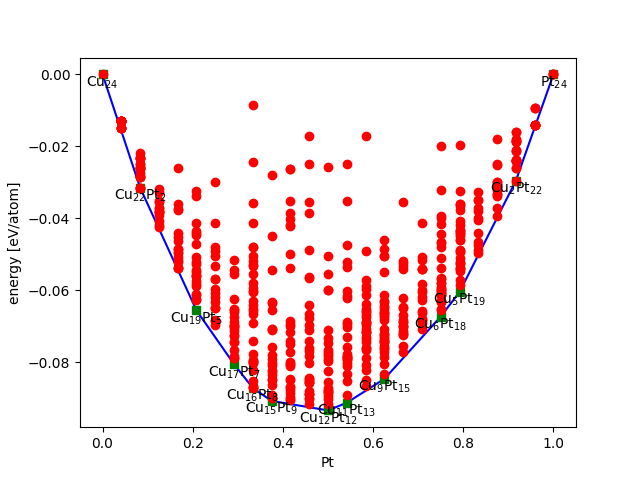
We can evaluate the results of the algorithm continuously while the database is being updated. We use the ase.phasediagram.PhaseDiagram to plot the convex hull. In the script below we retrieve the evaluated candidates and plot the convex hull. We also write a trajectory file with all the candidates that make up the convex hull. plot_convex_hull.py
import matplotlib.pyplot as plt
import numpy as np

from ase.db import connect
from ase.io import write
from ase.phasediagram import PhaseDiagram

db = connect('hull.db')

# Select the evaluated candidates and retrieve the chemical formula and mixing
# energy for the phase diagram
refs = []
dcts = list(db.select('relaxed=1'))
for dct in dcts:
    refs.append((dct.formula, -dct.raw_score))

pd = PhaseDiagram(refs)
ax = pd.plot(
    show=not True,  # set to True to show plot
    only_label_simplices=True,
)
plt.savefig('hull.png')

# View the simplices of the convex hull
simplices = []
toview = sorted(np.array(dcts)[pd.hull], key=lambda x: x.mass)
for dct in toview:
    simplices.append(dct.toatoms())

write('hull.traj', simplices)
All evaluated structures are put in the plot, if the number of points is disturbing the plot try to put only_plot_simplices=True instead of only_label_simplices=True.
We then view the structures on the convex hull by doing (on the command-line):
$ ase gui hull.traj
Customization of the algorithm#
So far we have a working algorithm but it is quite naive, let us make some extensions for increasing efficiency.
Exact duplicate identification#
Evaluating identical candidates is a risk when they are created by the operators, so in order not to waste computational resources it is important to implement a check for whether an identical calculation has been performed.
The list of elements in the candidate determines the structure completely, thus we can use that as a measure to see if an identical candidate has been evaluated:
for _ in range(pop_size):
  dup = True
  while dup:
      # Select parents for a new candidate
      parents = pop.get_two_candidates()

      # Select an operator and use it
      op = operation_selector.get_operator()
      offspring, desc = op.get_new_individual(parents)
      # An operator could return None if an offspring cannot be formed
      # by the chosen parents
      if offspring is None:
          continue

      atoms_string = ''.join(offspring.get_chemical_symbols())
      dup = db.is_duplicate(atoms_string=atoms_string)
Symmetric duplicate identification#
Having identical or very similar in the population will limit the diversity and cause premature convergence of the GA. We will try to prevent that by detecting if two structures are not identical in positions but instead symmetrically identical. For this we need a metric with which to characterize a structure, a symmetry tolerant fingerprint. There are many ways to achieve this and we will use a very simple average number of nearest neighbors, defined as:
where \(\#\text{Cu-Cu}\) is the number of Cu - Cu nearest neighbors and \(N_\text{Cu}\) is the total number of Cu atoms in the slab. This check can be performed at two points; either just after candidate creation before evaluation or after evaluation before potential inclusion into the population. We will use the latter method here and add a comparator to the population.
The nearest neighbor average is put in candidate.info['key_value_pairs'] as a string rounded off to two decimal points. Note this accuracy is fitting for this size slab, but need testing for other systems.
from ase.ga.utilities import get_nnmat_string

...

# The population instance is changed to
pop = RankFitnessPopulation(data_connection=db,
                            population_size=pop_size,
                            variable_function=get_comp,
                            comparator=StringComparator('nnmat_string'))

# Evaluating the starting population is changed to
while db.get_number_of_unrelaxed_candidates() > 0:
    a = db.get_an_unrelaxed_candidate()
    # The following line is added
    a.info['key_value_pairs']['nnmat_string'] = get_nnmat_string(a, 2, True)
    set_raw_score(a, -get_mixing_energy(a))
    db.add_relaxed_step(a)
pop.update()

...

# If a candidate is not an exact duplicate the nnmat should be calculated
# and added to the key_value_pairs
set_raw_score(offspring, -get_mixing_energy(offspring))
nnmat_string = get_nnmat_string(offspring, 2, True)
offspring.info['key_value_pairs']['nnmat_string'] = nnmat_string
offspring.info['key_value_pairs']['atoms_string'] = atoms_string
new_generation.append(offspring)
Problem specific mutation operators#
Sometimes it is necessary to introduce operators that force the GA to investigate certain areas of the phase space. The ase.ga.slab_operators.SymmetrySlabPermutation permutes the atoms in the slab to yield a more symmetric offspring. Note this requires spglib to be installed. Try it by:
from ase.ga.slab_operators import SymmetrySlabPermutation

oclist = [...
          (1, SymmetrySlabPermutation()),
          ...
         ]
Try to run the algorithm again to see if the number of evaluated structures goes down, but remember that the GA is non-deterministic so in order to compare efficiency of parameters one has to do statistics of many runs. The GA could also be run pool-based instead of generational, try to add each candidate to the database individually as they are evaluated and update the population after each addition, this should lower the total number of evaluations required to determine the convex hull.
Another extension to the tutorial could be to only allow different elements in the top three layers of a thicker slab. This would replicate a surface alloy.