
Electron transport#
The ase.transport module of ASE assumes the generic setup of the system
in question sketched below:
…  …
…
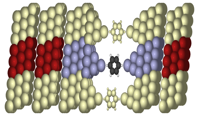
There is a central region (blue atoms plus the molecule) connected to two semi-infinite leads constructed by infinitely repeated principal layers (red atoms). The entire structure may be periodic in the transverse direction, which can be effectively sampled using k-points (yellowish atoms).
The system is described by a Hamiltonian matrix which must be represented in terms of a localized basis set such that each element of the Hamiltonian can be ascribed to either the left, central, or right region, or the coupling between these.
The Hamiltonian can thus be decomposed as:
where \(H_{L/R}\) describes the left/right principal layer, and \(H_C\) the central region. \(V_{L/R}\) is the coupling between principal layers, and from the principal layers into the central region. The central region must contain at least one principal layer on each side, and more if the potential has not converged to its bulk value at this size. The central region is assumed to be big enough that there is no direct coupling between the two leads. The principal layer must be so big that there is only coupling between nearest neighbor layers.
Having defined \(H_{L/R}\), \(V_{L/R}\), and \(H_C\), the elastic
transmission function can be determined using the Non-equilibrium
Green Function (NEGF) method. This is achieved by the class:
TransportCalculator (in
ase.transport.calculators) which makes no requirement on the origin of
these five matrices.
- class ase.transport.TransportCalculator(**kwargs)[source]#
Determine transport properties of a device sandwiched between two semi-infinite leads using a Green function method.
Create the transport calculator.
Parameters:
- h(N, N) ndarray
Hamiltonian matrix for the central region.
- s{None, (N, N) ndarray}, optional
Overlap matrix for the central region. Use None for an orthonormal basis.
- h1(N1, N1) ndarray
Hamiltonian matrix for lead1.
- h2{None, (N2, N2) ndarray}, optional
Hamiltonian matrix for lead2. You may use None if lead1 and lead2 are identical.
- s1{None, (N1, N1) ndarray}, optional
Overlap matrix for lead1. Use None for an orthonomormal basis.
- hc1{None, (N1, N) ndarray}, optional
Hamiltonian coupling matrix between the first principal layer in lead1 and the central region.
- hc2{None, (N2, N} ndarray), optional
Hamiltonian coupling matrix between the first principal layer in lead2 and the central region.
- sc1{None, (N1, N) ndarray}, optional
Overlap coupling matrix between the first principal layer in lead1 and the central region.
- sc2{None, (N2, N) ndarray}, optional
Overlap coupling matrix between the first principal layer in lead2 and the central region.
- energies{None, array_like}, optional
Energy points for which calculated transport properties are evaluated.
- eta{1.0e-5, float}, optional
Infinitesimal for the central region Green function.
- eta1/eta2{1.0e-5, float}, optional
Infinitesimal for lead1/lead2 Green function.
- align_bf{None, int}, optional
Use align_bf=m to shift the central region by a constant potential such that the m’th onsite element in the central region is aligned to the m’th onsite element in lead1 principal layer.
- logfile{None, str}, optional
Write a logfile to file with name \(logfile\). Use ‘-’ to write to std out.
- eigenchannels: {0, int}, optional
Number of eigenchannel transmission coefficients to calculate.
- pdos{None, (N,) array_like}, optional
Specify which basis functions to calculate the projected density of states for.
- dos{False, bool}, optional
The total density of states of the central region.
- box: XXX
YYY
If hc1/hc2 are None, they are assumed to be identical to the coupling matrix elements between neareste neighbor principal layers in lead1/lead2.
Examples:
>>> import numpy as np
>>> h = np.array((0,)).reshape((1,1))
>>> h1 = np.array((0, -1, -1, 0)).reshape(2,2)
>>> energies = np.arange(-3, 3, 0.1)
>>> calc = TransportCalculator(h=h, h1=h1, energies=energies)
>>> T = calc.get_transmission()
This module is stand-alone in the sense that it makes no requirement on the origin of these five matrices. They can be model Hamiltonians or derived from different kinds of electronic structure codes.
For an example of how to use the ase.transport module, see section 9.2
in the ASE-paper:
J. Phys. Condens. Matter: The Atomic Simulation Environment | A Python library for working with atoms (7 June 2017).