Visualization#
- ase.visualize.view(atoms, data=None, viewer=None, repeat=None)#
This provides an interface to various visualization tools, such as
ase.gui, RasMol, VMD, gOpenMol, Avogadro, ParaView or NGLView. The default viewer is
the ase.gui, described in the ase.gui module. The simplest invocation
is:
>>> from ase.visualize import view
>>> view(atoms)
where atoms is any Atoms object. Alternative viewers
can be used by specifying the optional keyword viewer=... - use one of
‘ase.gui’, ‘gopenmol’, ‘vmd’, ‘rasmol’, ‘paraview’, ‘ngl’. The VMD and Avogadro viewers can
take an optional data argument to show 3D data, such as charge density:
>>> view(atoms, viewer='VMD', data=...)
The nglview viewer additionally supports any indexible sequence of Atoms
objects, e.g. lists of structures and Trajectory objects.
If you do not wish to open an interactive gui, but rather visualize
your structure by dumping directly to a graphics file; you can use the
write command of the ase.io module, which can write ‘eps’,
‘png’, and ‘pov’ files directly, like this:
>>> from ase.io import write
>>> write('image.png', atoms)
It is also possible to plot directly to a Matplotlib subplot object, which allows for a large degree of customisability. More information.
Viewer for Jupyter notebooks#
A simple viewer based on X3D is built into ASE, which should work on modern browsers without additional packages, by typing the following command into a Jupyter notebook:
>>> view(atoms, viewer='x3d')
For a more feature-rich viewer, nglview is a dedicated viewer for the Jupyter notebook interface. It uses an embeddable NGL WebGL molecular viewer. The viewer works only in the web browser environment and embeds the live javascript output into the notebook. To utilize this functionality you need to have NGLView and ipywidgets packages installed in addition to the Jupyter notebook.
The basic usage provided by the ase.visualize.view() function exposes
only small fraction of the NGL widget capabilities. The simplest form:
>>> view(atoms, viewer='ngl')
creates interactive ngl viewer widget with the few additional control widgets
added on the side. The object returned by the above call is a reference to
the \(.gui\) member of the ase.visualize.nglview.NGLDisplay containing
actual viewer (\(.view\) member), a reference to control widgets box
(\(.control_box\) member) and
ase.visualize.view.nglview.NGLDisplay.custom_colors() method. The
notebook interface is not blocked by the above call and the returned object
may be further manipulated by the following code in the separate cell (the
\(\_\) variable contains output from the previous cell):
>>> v=_
>>> v.custom_colors({'Mn':'green','As':'blue'})
>>> v.view._remote_call("setSize", target="Widget", args=["400px", "400px"])
>>> v.view.center_view()
>>> v.view.background='#ffc'
>>> v.view.parameters=dict(clipDist=-200)
The \(.view\) member exposes full API of the NGLView widget. The
\(.control_box\) member is a ipywidgets.HBox containing
nglview.widget.NGLWidget and ipywidgets.VBox with control
widgets. For the full documentation of these objects consult the NGLView,
NGL and ipywidgets websites.
- class ase.visualize.ngl.NGLDisplay(atoms, xsize=500, ysize=500)[source]#
Structure display class
Provides basic structure/trajectory display in the notebook and optional gui which can be used to enhance its usability. It is also possible to extend the functionality of the particular instance of the viewer by adding further widgets manipulating the structure.
- ase.visualize.ngl.view_ngl(atoms, data=None, repeat=None, w=500, h=500)[source]#
Returns the nglviewer + some control widgets in the VBox ipywidget. The viewer supports any Atoms objectand any sequence of Atoms objects. The returned object has two shortcuts members:
- .view:
nglviewer ipywidget for direct interaction
- .control_box:
VBox ipywidget containing view control widgets
Plotting iso-surfaces with Mayavi#
The ase.visualize.mlab.plot() function can be used from the
command-line:
$ python -m ase.visualize.mlab abc.cube
to plot data from a cube-file or alternatively a wave function or an electron density from a calculator restart file:
$ python -m ase.visualize.mlab -C gpaw abc.gpw
Options:
- -h, --help
show this help message and exit
- -n INDEX, --band-index=INDEX
Band index counting from zero.
- -s SPIN, --spin-index=SPIN
Spin index: zero or one.
- -e, --electrostatic-potential
Plot the electrostatic potential.
- -c CONTOURS, --contours=CONTOURS
Use “-c 3” for 3 contours or “-c -0.5,0.5” for specific values. Default is four contours.
- -r REPEAT, --repeat=REPEAT
Example: “-r 2,2,2”.
- -C NAME, --calculator-name=NAME
Name of calculator.
Matplotlib#
>>> import matplotlib.pyplot as plt
>>> from ase.visualize.plot import plot_atoms
>>> from ase.lattice.cubic import FaceCenteredCubic
>>> slab = FaceCenteredCubic('Au', size=(2, 2, 2))
>>> fig, ax = plt.subplots()
>>> plot_atoms(slab, ax, radii=0.3, rotation=('90x,45y,0z'))
>>> fig.savefig("ase_slab.png")
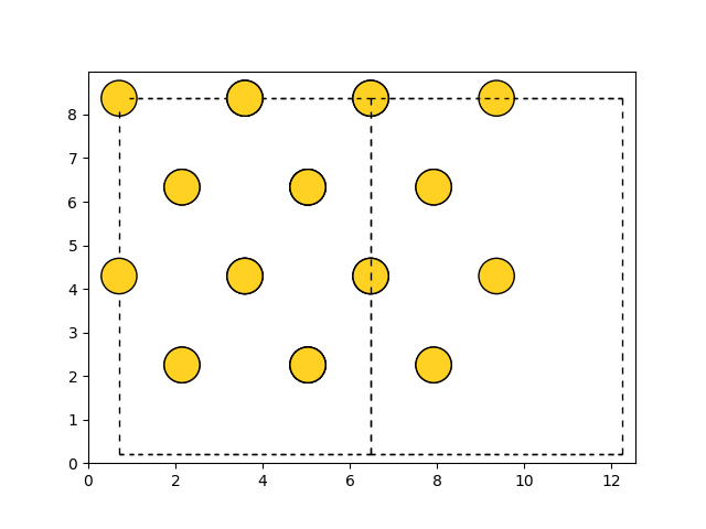
The data is plotted directly to a Matplotlib subplot object, giving a large degree of customizability.
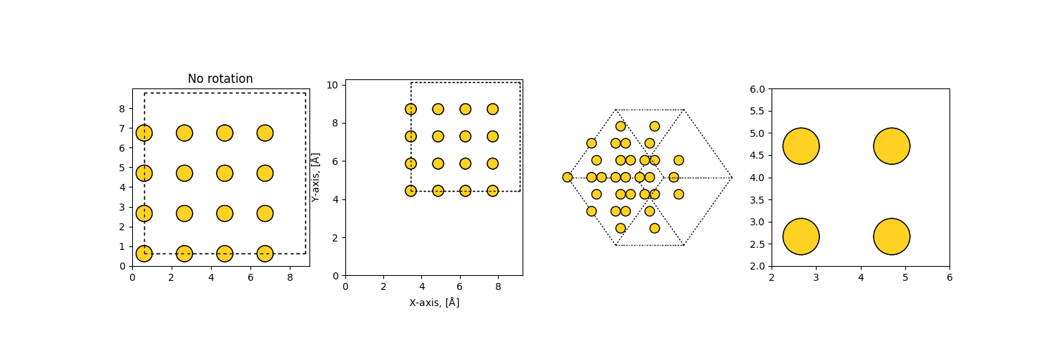
>>> import matplotlib.pyplot as plt
>>> from ase.visualize.plot import plot_atoms
>>> from ase.lattice.cubic import FaceCenteredCubic
>>> slab = FaceCenteredCubic('Au', size=(2, 2, 2))
>>> fig, axarr = plt.subplots(1, 4, figsize=(15, 5))
>>> plot_atoms(slab, axarr[0], radii=0.3, rotation=('0x,0y,0z'))
>>> plot_atoms(slab, axarr[1], scale=0.7, offset=(3, 4), radii=0.3, rotation=('0x,0y,0z'))
>>> plot_atoms(slab, axarr[2], radii=0.3, rotation=('45x,45y,0z'))
>>> plot_atoms(slab, axarr[3], radii=0.3, rotation=('0x,0y,0z'))
>>> axarr[0].set_title("No rotation")
>>> axarr[1].set_xlabel("X-axis, [$\mathrm{\AA}$]")
>>> axarr[1].set_ylabel("Y-axis, [$\mathrm{\AA}$]")
>>> axarr[2].set_axis_off()
>>> axarr[3].set_xlim(2, 6)
>>> axarr[3].set_ylim(2, 6)
>>> fig.savefig("ase_slab_multiple.png")
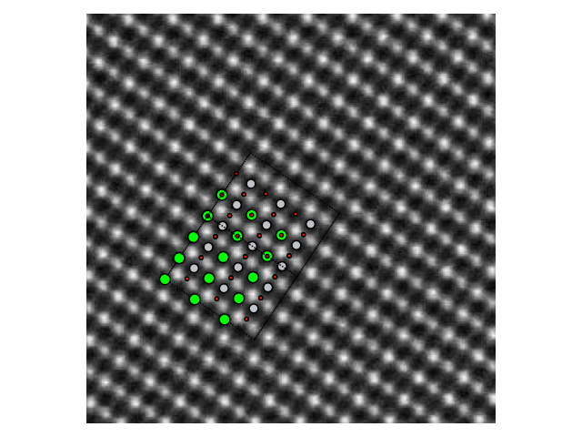
>>> stem_image = mpimg.imread("stem_image.jpg")
>>> atom_pos = [(0.0, 0.0, 0.0), (0.5, 0.5, 0.5), (0.5, 0.5, 0.0)]
>>> srtio3 = crystal(['Sr','Ti','O'], atom_pos, spacegroup=221, cellpar=3.905, size=(3, 3, 3))
>>> fig, ax = plt.subplots()
>>> ax.imshow(stem_image, cmap='gray')
>>> plot_atoms(srtio3, ax, radii=0.3, scale=6.3, offset=(47, 54), rotation=('90x,45y,56z'))
>>> ax.set_xlim(0, stem_image.shape[0])
>>> ax.set_ylim(0, stem_image.shape[1])
>>> ax.set_axis_off()
>>> fig.tight_layout()
>>> fig.savefig("iomatplotlib3.png")