Nonlinear optical response of an extended system

A short introduction

The nonlinear optical (NLO) response of an extended system can be obtained from its ground state electronic structure. Due to large computional cost, the local field effect effect is neglected. Hence, the NLO response is only frequency-dependent. The NLO response can be descibed by nonlinear susceptibility tensors. There are numerious NLO processes, depending on the number of photons involved in the process.

The second-harmonic generation (SHG) is a NLO process in which two photons at the frequency of \(\omega\) generate a photon at the frequency of \(2\omega\). The SHG response is characterized by the second-order (quadratic) susceptibility tensor, defined via

\[P_{\gamma}(t) = \sum_{\alpha\beta} \chi_{\gamma\alpha\beta}^{(2)}(\omega,\omega) E_{\alpha}E_{\beta} e^{-2i\omega t}+\textrm{c.c.}\]

where \(\alpha,\beta,\gamma={x,y,z}\) denote the Cartesian coordinate axes, and \(P_{\alpha}\) and \(E_{\alpha}\) are the polarization and electric fields, respectivly. For bulk systems, \(\chi_{\gamma\alpha\beta}^{(2)}\) is expressed in the units of m/V. The details of computing \(\chi_{\gamma\alpha\beta}^{(2)}\) is documented in Ref. [1].

Example 1: SHG spectrum of semiconductor: Monolayer MoS2

To compute the SHG spectrum of given structure, 3 steps are performed:

1. Ground state calculation

import numpy as np
from ase.build import mx2

from gpaw import GPAW, PW, FermiDirac
from gpaw.nlopt.matrixel import make_nlodata
from gpaw.nlopt.shg import get_shg

# Make the structure and add the vaccum around the layer
atoms = mx2(formula='MoS2', a=3.16, thickness=3.17, vacuum=5.0)
atoms.center(vacuum=15, axis=2)

# GPAW parameters:
nk = 40
params_gs = {
    'mode': PW(800),
    'symmetry': {'point_group': False, 'time_reversal': True},
    'nbands': 'nao',
    'convergence': {'bands': -10},
    'parallel': {'domain': 1},
    'occupations': FermiDirac(width=0.05),
    'kpts': {'size': (nk, nk, 1), 'gamma': True},
    'xc': 'PBE',
    'txt': 'gs.txt'
}

# Ground state calculation:
gs_name = 'gs.gpw'
calc = GPAW(**params_gs)
atoms.calc = calc
atoms.get_potential_energy()
atoms.calc.write(gs_name, mode='all')

In this script a normal ground state calculation is performed with a coarse k-point grid. For a smoother spectrum, a finer mesh should be employed. Please note that the current implementation of the nonlinear optics module only supports the plane-wave basis set.

2. Get the required matrix elements from the ground state

   Here, the matrix elements of the momentum operator are computed. Afterwards, all required quantities such as energies, occupations, and momentum matrix elements are saved in a file (‘mml.npz’). The ground state file 'gs.gpw' can be deleted after this step.

   # Calculate momentum matrix elements:
   nlodata = make_nlodata(gs_name)
   nlodata.write('mml.npz')
   

   Note

   After writing the momentum matrix elements to your harddisk, you can load them quickly through:

   from gpaw.nlopt.basic import NLOData
   nlodata = NLOData.load('mml.npz', comm=world)
   

   Note

   Two optional parameters are available in the gpaw.nlopt.matrixel.make_nlodata() function: ni and nf as the first and last bands used for calculations of SHG.

3. Compute the SHG spectrum

   In this step, the SHG spectrum is calculated using the saved data, and there are two well-known gauges that can be used: the length gauge and the velocity gauge. Formally, they are equivalent but they may generate different results. The SHG susceptibility is computed in both gauges and saved.

   A broadening is necessary to obtain smooth graphs, and here 50 meV has been used.

   The SHG susceptibility is a rank-3 symmetric tensor with at most 18 independent components. In addition, the point group symmetry reduces the number of independent tensor elements. Monolayer MoS2 has only one independent tensor element: yyy.

   # Shift parameters:
   eta = 0.05  # Broadening in eV
   w_ls = np.linspace(0, 6, 500)  # in eV
   pol = 'yyy'
   
   # LG calculation
   shg_name1 = 'shg_' + pol + '_lg.npy'
   get_shg(
       nlodata, freqs=w_ls, eta=eta, pol=pol,
       gauge='lg', out_name=shg_name1)
   
   # VG calculation
   shg_name2 = 'shg_' + pol + '_vg.npy'
   get_shg(
       nlodata, freqs=w_ls, eta=eta, pol=pol,
       gauge='vg', out_name=shg_name2)
   

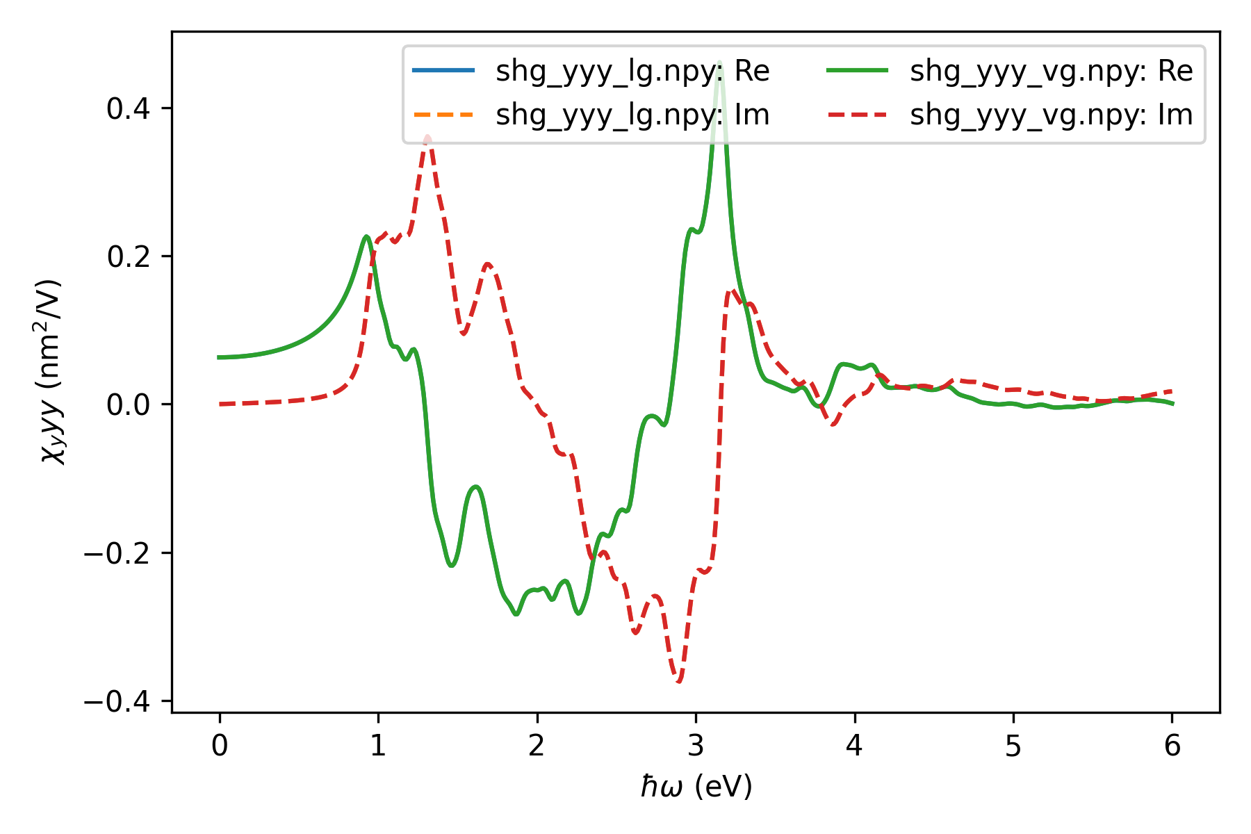
Result

We will now plot the calculated SHG spectra. Both real and imaginary parts of the computed SHG susceptibilities, obtained from two gauges are shown. The gauge invariance is confirmed from the calculation.

Note that the bulk susceptibility (with SI units of m/V) is ill-defined for 2D materials, since the crystal volume cannot be defined without ambiguity. Instead, the sheet susceptibility, expressed in unit of m\(^2\)/V, is an unambiguous quantity for 2D materials. Hence, the bulk susceptibility is transformed to the unambiguous sheet susceptibility by multiplying with the width of the unit cell in the \(z\)-direction.

import numpy as np
import matplotlib.pyplot as plt
from ase.io import read

# Plot and save both spectra
atoms = read('gs.txt')
cell = atoms.get_cell()
cellsize = atoms.cell.cellpar()
mult = cellsize[2] * 1e-10  # Make the sheet susceptibility
legls = []
res_name = ['shg_yyy_lg.npy', 'shg_yyy_vg.npy']
plt.figure(figsize=(6.0, 4.0), dpi=300)
for ii, name in enumerate(res_name):
    # Load the data
    shg = np.load(name)
    w_l = shg[0].real
    plt.plot(w_l, np.real(mult * shg[1] * 1e18), '-')
    plt.plot(w_l, np.imag(mult * shg[1] * 1e18), '--')
    legls.append(f'{name}: Re')
    legls.append(f'{name}: Im')
    plt.xlabel(r'$\hbar\omega$ (eV)')
    plt.ylabel(r'$\chi_{yyy}$ (nm$^2$/V)')
    plt.legend(legls, ncol=2)
plt.tight_layout()
plt.savefig('shg.png', dpi=300)

The figure shown here is generated from scripts: shg_MoS2.py and shg_plot.py. It takes roughly 15 minutes with 16 CPUs on Intel Xeon X5570 2.93GHz.

Technical details

There are few points about the implementation that we emphasize:

• The code is parallelized over k-points.

• The code employs only the time reversal symmetry to improve the speed.

• Refer to [1] for the details on the NLO theory.

Useful tips

It’s important to converge the results with respect to:

• nbands

• nkpt (number of k-points in gs calc.)

• eta

• ecut

• ftol

• vacuum (if there is)

API

gpaw.nlopt.matrixel.make_nlodata(calc, spin_string='all', ni=None, nf=None)

This function calculates and returns all required NLO data: w_sk, f_skn, E_skn, p_skvnn.

Parameters:

• calc (gpaw.new.ase_interface.ASECalculator | str | pathlib.Path) – Calculator or string/path pointing to a .gpw file.

• spin_string (str) – String denoting which spin channels to include (‘all’, ‘s0’ , ‘s1’).

• ni (Optional[int]) – First band to compute the mml.

• nf (Optional[int]) – Last band to compute the mml (relative to number of bands for nf <= 0).

Returns:

Data object carrying required matrix elements for NLO calculations.

Return type:

NLOData

gpaw.nlopt.shg.get_shg(nlodata, freqs=[1.0], eta=0.05, pol='yyy', eshift=0.0, gauge='lg', ftol=0.0001, Etol=1e-06, band_n=None, out_name='shg.npy')

Calculate SHG spectrum within the independent particle approximation (IPA) for nonmagnetic semiconductors.

Output: shg.npy file with numpy array containing the spectrum and frequencies.

Parameters:

• nlodata – Data object of class NLOData. Contains energies, occupancies and momentum matrix elements.

• freqs – Excitation frequency array (a numpy array or list).

• eta – Broadening, a number or an array (default 0.05 eV).

• pol – Tensor element (default ‘yyy’).

• gauge – Choose the gauge (‘lg’ or ‘vg’).

• Etol – Tol. in energy and fermi to consider degeneracy.

• ftol – Tol. in energy and fermi to consider degeneracy.

• band_n – List of bands in the sum (default 0 to nb).

• out_name – Output filename (default ‘shg.npy’).

gpaw.nlopt.linear.get_chi_tensor(nlodata, freqs=[1.0], eta=0.05, ftol=0.0001, Etol=1e-06, eshift=0.0, band_n=None, out_name=None)

Calculate full linear susceptibility tensor for nonmagnetic semiconductors; array will be saved to disk if out_name is given.

Parameters:

• nlodata – Data object of type NLOData.

• freqs – Excitation frequency array (a numpy array or list).

• eta – Broadening, a number or an array (default 0.05 eV).

• Etol – Tolerance in energy and occupancy to consider degeneracy.

• ftol – Tolerance in energy and occupancy to consider degeneracy.

• eshift – Bandgap correction.

• band_n – List of bands in the sum (default 0 to nb).

• out_name – If it is given: output filename.

Returns:

Full linear susceptibility tensor (3, 3, nw).

Return type:

np.ndarray

gpaw.nlopt.shift.get_shift(nlodata, freqs=[1.0], eta=0.05, pol='yyy', eshift=0.0, ftol=0.0001, Etol=1e-06, band_n=None, out_name='shift.npy')

Calculate RPA shift current for nonmagnetic semiconductors.

Parameters:

• nlodata – Data object of class NLOData.

• freqs – Excitation frequency array (a numpy array or list).

• eta – Broadening, a number or an array (default 0.05 eV).

• pol – Tensor element (default ‘yyy’).

• Etol – Tolerance in energy and fermi to consider degeneracy.

• ftol – Tolerance in energy and fermi to consider degeneracy.

• band_n – List of bands in the sum (default 0 to nb).

• out_name – Output filename (default ‘shift.npy’).

Returns:

Numpy array containing the spectrum and frequencies.

Return type:

np.ndarray

[1] (1,2)

A. Taghizadeh, K. S. Thygesen and T. G. Pedersen Arxiv, 2010.11596 (2020)