Simulating an XAS spectrum
First we must create a core hole setup. This can be done with the gpaw-setup command:
gpaw-setup -f PBE N --name hch1s --core-hole=1s,0.5
or you can write a small script to do it:
from gpaw.atom.generator import Generator
from gpaw.atom.configurations import parameters

# Generate setups with 0.5, 1.0, 0.0 core holes in 1s
elements = ['O', 'C', 'N']
coreholes = [0.5, 1.0, 0.0]
names = ['hch1s', 'fch1s', 'xes1s']
functionals = ['LDA', 'PBE']

for el in elements:
    for name, ch in zip(names, coreholes):
        for funct in functionals:
            g = Generator(el, scalarrel=True, xcname=funct,
                          corehole=(1, 0, ch), nofiles=True)
            g.run(name=name, **parameters[el])
Set the location of setups as described here: Installation of PAW datasets.
Spectrum calculation using unoccupied states
We do a “ground state” calculation with a core hole. Use a lot of unoccupied states.
from math import pi, cos, sin
from ase import Atoms
from gpaw import GPAW, setup_paths
setup_paths.insert(0, '.')

a = 12.0  # use a large cell

d = 0.9575
t = pi / 180 * 104.51
atoms = Atoms('OH2',
              [(0, 0, 0),
               (d, 0, 0),
               (d * cos(t), d * sin(t), 0)],
              cell=(a, a, a))
atoms.center()
calc = GPAW(mode='fd',
            nbands=-30,
            h=0.2,
            txt='h2o_xas.txt',
            setups={'O': 'hch1s'})
# the number of unoccupied stated will determine how
# high you will get in energy

atoms.calc = calc
e = atoms.get_potential_energy()

calc.write('h2o_xas.gpw')
To get the absolute energy scale we do a Delta Kohn-Sham calculation
where we compute the total energy difference between the ground state
and the first core excited state. The excited state should be spin
polarized and to fix the occupation to a spin up core hole and an
electron in the lowest unoccupied spin up state (singlet) we must set
the magnetic moment to one on the atom with the hole and fix the total
magnetic moment with occupations=FermiDirac(0.0, fixmagmom=True):
from math import pi, cos, sin
from ase import Atoms
from ase.parallel import paropen
from gpaw import GPAW, setup_paths, FermiDirac
setup_paths.insert(0, '.')

a = 12.0  # use a large cell

d = 0.9575
t = pi / 180 * 104.51
atoms = Atoms('OH2',
              [(0, 0, 0),
               (d, 0, 0),
               (d * cos(t), d * sin(t), 0)],
              cell=(a, a, a))
atoms.center()

calc1 = GPAW(mode='fd',
             h=0.2,
             txt='h2o_gs.txt',
             xc='PBE')
atoms.calc = calc1
e1 = atoms.get_potential_energy() + calc1.get_reference_energy()

calc2 = GPAW(mode='fd',
             h=0.2,
             txt='h2o_exc.txt',
             xc='PBE',
             charge=-1,
             spinpol=True,
             occupations=FermiDirac(0.0, fixmagmom=True),
             setups={0: 'fch1s'})
atoms[0].magmom = 1
atoms.calc = calc2
e2 = atoms.get_potential_energy() + calc2.get_reference_energy()

with paropen('dks.result', 'w') as fd:
    print('Energy difference:', e2 - e1, file=fd)
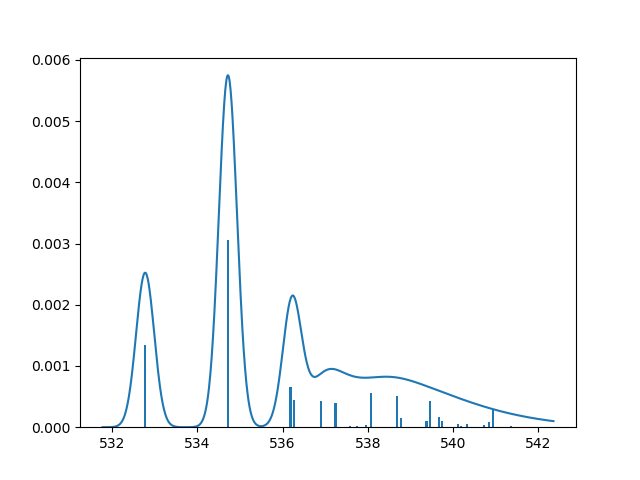
Plot the spectrum:
from gpaw import GPAW, setup_paths
from gpaw.xas import XAS
import matplotlib.pyplot as plt

setup_paths.insert(0, '.')

dks_energy = 532.774  # from dks calcualtion

calc = GPAW('h2o_xas.gpw')

xas = XAS(calc, mode='xas')
x, y = xas.get_spectra(fwhm=0.5, linbroad=[4.5, -1.0, 5.0])
x_s, y_s = xas.get_spectra(stick=True)

shift = dks_energy - x_s[0]  # shift the first transition

y_tot = y[0] + y[1] + y[2]
y_tot_s = y_s[0] + y_s[1] + y_s[2]

plt.plot(x + shift, y_tot)
plt.bar(x_s + shift, y_tot_s, width=0.05)
plt.savefig('xas_h2o_spectrum.png')
Haydock recursion method
For systems in the condensed phase it is much more efficient to use the Haydock recursion method to calculate the spectrum, thus avoiding to determine many unoccupied states. First we do a core hole calculation with enough k-points to converge the ground state density. Then we compute the recursion coefficients with a denser k-point mesh to converge the uncoccupied DOS. A Delta Kohn-Sham calculation can be done for the gamma point, and the shift is made so that the first unoccupied eigenvalue at the gamma point ends up at the computed total energy difference.
from ase import Atoms
from gpaw import GPAW, setup_paths

setup_paths.insert(0, '.')

name = 'diamond333_hch'

a = 3.574

atoms = Atoms('C8', [(0, 0, 0),
                     (1, 1, 1),
                     (2, 2, 0),
                     (3, 3, 1),
                     (2, 0, 2),
                     (0, 2, 2),
                     (3, 1, 3),
                     (1, 3, 3)],
              cell=(4, 4, 4),
              pbc=True)

atoms.set_cell((a, a, a), scale_atoms=True)
atoms *= (3, 3, 3)

calc = GPAW(mode='fd',
            h=0.2,
            txt=name + '.txt',
            xc='PBE',
            setups={0: 'hch1s'})

atoms.calc = calc

e = atoms.get_potential_energy()

calc.write(name + '.gpw')
Compute recursion coefficients:
from gpaw import GPAW, setup_paths
from gpaw.xas import RecursionMethod

setup_paths.insert(0, '.')

name = 'diamond333_hch'

calc = GPAW(name + '.gpw',
            kpts=(6, 6, 6),
            txt=name + '_rec.txt')
calc.initialize()
calc.set_positions()

r = RecursionMethod(calc)
r.run(600)

r.run(1400,
      inverse_overlap='approximate')

r.write(name + '_600_1400a.rec',
        mode='all')
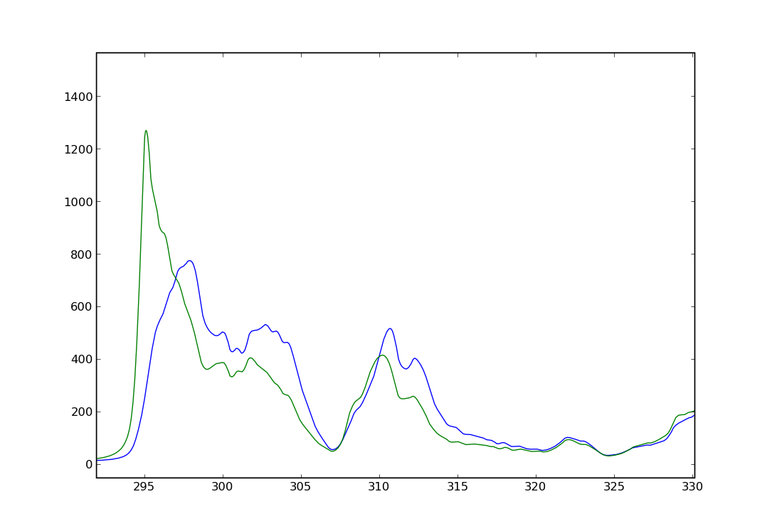
Compute the spectrum with the get_spectra method. delta is the HWHM (should we change it to FWHM???) width of the lorentzian broadening, and fwhm is the FWHM of the Gaussian broadening.
sys.setrecursionlimit(10000)

name='diamond333_hch_600_1400a.rec'
x_start=-20
x_end=100
dx=0.01
x_rec = x_start + npy.arange(0, x_end - x_start ,dx)

r = RecursionMethod(filename=name)
y = r.get_spectra(x_rec, delta=0.4, fwhm=0.4 )
y2 = sum(y)

p.plot(x_rec + 273.44,y2)
p.show()
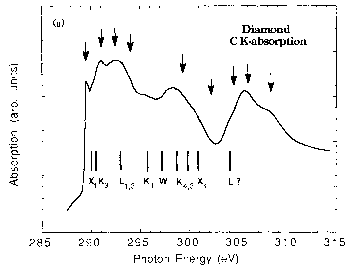
Below the calculated spectrum of Diamond with half and full core holes are shown along with the experimental spectrum.
XES
To compute XES, first do a ground state calcualtion with an 0.0 core hole (an ‘xes1s’ setup as created above ). The system will not be charged so the setups can be placed on all atoms one wants to calculte XES for. Since XES probes the occupied states no unoccupied states need to be determined. Calculate the spectrum with
xas = XAS(calc, mode='xes', center=n)
Where n is the number of the atom in the atoms object, the center keyword is only necessary if there are more than one xes setup. The spectrum can be shifted by putting the first transition to the fermi level, or to compute the total energy diffrence between the core hole state and the state with a valence hole in HOMO.
Further considerations
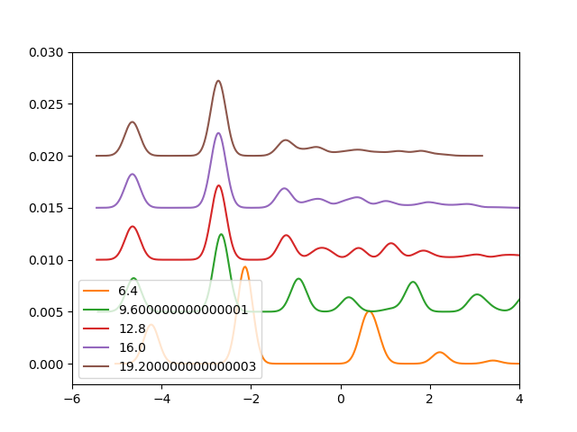
For XAS: Gridspacing can be set to the default value. The shape of the spectrum is quite insensitive to the functional used, the DKS shifts are more sensitive. The absolute energy position can be shifted so that the calculated XPS energy matches the expreimental value [Leetmaa2006]. Use a large box, see convergence with box size for a water molecule below:
import numpy as np
from ase.build import molecule
from gpaw import GPAW, setup_paths
setup_paths.insert(0, '.')

atoms = molecule('H2O')

h = 0.2

for L in np.arange(4, 14, 2) * 8 * h:
    atoms.set_cell((L, L, L))
    atoms.center()
    calc = GPAW(mode='fd',
                xc='PBE',
                h=h,
                nbands=-40,
                eigensolver='cg',
                setups={'O': 'hch1s'})
    atoms.calc = calc
    e1 = atoms.get_potential_energy()
    calc.write(f'h2o_hch_{L:.1f}.gpw')
and plot it
import numpy as np
import matplotlib.pyplot as plt

from gpaw import GPAW, setup_paths
from gpaw.xas import XAS

setup_paths.insert(0, '.')

h = 0.2

offset = 0.0
for L in np.arange(4, 14, 2) * 8 * h:
    calc = GPAW(f'h2o_hch_{L:.1f}.gpw')
    xas = XAS(calc)
    x, y = xas.get_spectra(fwhm=0.4)
    plt.plot(x, sum(y) + offset, label=f'{L:.1f}')
    offset += 0.005

plt.legend()
plt.xlim(-6, 4)
plt.ylim(-0.002, 0.03)
plt.savefig('h2o_xas_box.png')
Chemical bonding on surfaces probed by X-ray emission spectroscopy and density functional theory, A. Nilsson and L. G. M. Pettersson, Surf. Sci. Rep. 55 (2004) 49-167