Quasi-particle spectrum in the GW approximation: tutorial
For a brief introduction to the GW theory and the details of its implementation in GPAW, see Quasi-particle spectrum in the GW approximation: theory.
More information can be found here:
F. Hüser, T. Olsen, and K. S. Thygesen
Quasiparticle GW calculations for solids, molecules, and two-dimensional materials
Physical Review B, Vol. 87, 235132 (2013)
Quasi-particle spectrum of bulk diamond
In the first part of the tutorial, the G0W0 calculator is introduced and the quasi-particle spectrum of bulk diamond is calculated.
Note
This tutorial has been updated Jun 17th 2024 to include Wigner-Seitz truncation method for the Coulomb kernel, which greatly improves convergence.
Groundstate calculation
First, we need to do a regular groundstate calculation. We do this in plane wave mode and choose the LDA exchange-correlation functional. In order to keep the computational efforts small, we start with (3x3x3) k-points and a plane wave basis up to 300 eV.
from ase.build import bulk
from gpaw import GPAW, FermiDirac
from gpaw import PW

a = 3.567
atoms = bulk('C', 'diamond', a=a)

calc = GPAW(mode=PW(300),  # energy cutoff for plane wave basis (in eV)
            kpts={'size': (3, 3, 3), 'gamma': True},
            xc='LDA',
            occupations=FermiDirac(0.001),
            parallel={'domain': 1},
            txt='C_groundstate.txt')

atoms.calc = calc
atoms.get_potential_energy()

calc.diagonalize_full_hamiltonian()  # determine all bands
calc.write('C_groundstate.gpw', 'all')  # write out wavefunctions
It takes a few seconds on a single CPU. The last line in the script creates a .gpw file which contains all the informations of the system, including the wavefunctions.
Note
You can change the number of bands to be written out by using
calc.diagonalize_full_hamiltonian(nbands=...).
This can be useful if not all bands are needed.
The GW calculator
Next, we set up the G0W0 calculator and calculate the quasi-particle spectrum
for all the k-points present in the irreducible Brillouin zone from the ground
state calculation and the specified bands.
In this case, each carbon atom has 4 valence electrons and the bands are double
occupied. Setting bands=(3,5) means including band index 3 and 4 which is
the highest occupied band and the lowest unoccupied band.
from gpaw.response.g0w0 import G0W0

gw = G0W0(calc='C_groundstate.gpw',
          nbands=30,  # number of bands for calculation of self-energy
          bands=(3, 5),          # VB and CB
          ecut=20.0,             # plane-wave cutoff for self-energy
          integrate_gamma='WS',  # Use supercell Wigner-Seitz truncation for W.
          filename='C-g0w0')
gw.calculate()
It takes about 30 seconds on a single CPU for the
calculate() method to finish:
- G0W0.calculate()
Starts the G0W0 calculation.
Returns a dict with the results with the following key/value pairs:
key
value
fOccupation numbers
epsKohn-Sham eigenvalues in eV
vxcExchange-correlation contributions in eV
exxExact exchange contributions in eV
sigmaSelf-energy contributions in eV
dsigmaSelf-energy derivatives
sigma_eSelf-energy contributions in eV used for ecut extrapolation
ZRenormalization factors
qpQuasi particle (QP) energies in eV
iqpGW0/GW: QP energies for each iteration in eV
All the values are
ndarray’s of shape (spins, IBZ k-points, bands).
The dictionary is stored in C-g0w0_results.pckl. From the dict it is
for example possible to extract the direct bandgap at the Gamma point:
import pickle

results = pickle.load(open('C-g0w0_results_GW.pckl', 'rb'))
direct_gap = results['qp'][0, 0, -1] - results['qp'][0, 0, -2]

print('Direct bandgap of C:', direct_gap)
with the result: 7.11 eV.
The possible input parameters of the G0W0 calculator are listed here:
- class gpaw.response.g0w0.G0W0(calc, filename='gw', ecut=150.0, ecut_extrapolation=False, xc='RPA', ppa=False, E0=27.211386024367243, eta=0.1, nbands=None, bands=None, relbands=None, frequencies=None, domega0=None, omega2=None, nblocks=1, nblocksmax=False, kpts=None, world=MPIComm(size=1, rank=0), timer=None, fxc_mode='GW', truncation=None, integrate_gamma='sphere', q0_correction=False, do_GW_too=False, **kwargs)[source]
G0W0 calculator wrapper.
The G0W0 calculator is used to calculate the quasi particle energies through the G0W0 approximation for a number of states.
- Parameters:
calc – Filename of saved calculator object.
filename (str) – Base filename of output files.
kpts (list) – List of indices of the IBZ k-points to calculate the quasi particle energies for.
bands – Range of band indices, like (n1, n2), to calculate the quasi particle energies for. Bands n where n1<=n<n2 will be calculated. Note that the second band index is not included.
relbands – Same as bands except that the numbers are relative to the number of occupied bands. E.g. (-1, 1) will use HOMO+LUMO.
frequencies – Input parameters for the nonlinear frequency descriptor.
ecut (float) – Plane wave cut-off energy in eV.
ecut_extrapolation (bool or list) – If set to True an automatic extrapolation of the selfenergy to infinite cutoff will be performed based on three points for the cutoff energy. If an array is given, the extrapolation will be performed based on the cutoff energies given in the array.
nbands (int) – Number of bands to use in the calculation. If None, the number will be determined from :ecut: to yield a number close to the number of plane waves used.
ppa (bool) – Sets whether the Godby-Needs plasmon-pole approximation for the dielectric function should be used.
xc (str) – Kernel to use when including vertex corrections.
fxc_mode (str) – Where to include the vertex corrections; polarizability and/or self-energy. ‘GWP’: Polarizability only, ‘GWS’: Self-energy only, ‘GWG’: Both.
do_GW_too (bool) – When carrying out a calculation including vertex corrections, it is possible to get the standard GW results at the same time (almost for free).
truncation (str) – Coulomb truncation scheme. Can be either 2D, 1D, or 0D.
integrate_gamma (str or dict) –
Method to integrate the Coulomb interaction.
The default is ‘sphere’. If ‘reduced’ key is not given, it defaults to False.
- {‘type’: ‘sphere’} or ‘sphere’:
Analytical integration of q=0, G=0 1/q^2 integrand in a sphere matching the volume of a single q-point. Used to be integrate_gamma=0.
- {‘type’: ‘reciprocal’} or ‘reciprocal’:
Numerical integration of q=0, G=0 1/q^2 integral in a volume resembling the reciprocal cell (parallelpiped). Used to be integrate_gamma=1.
- {‘type’: ‘reciprocal’, ‘reduced’:True} or ‘reciprocal2D’:
Numerical integration of q=0, G=0 1/q^2 integral in a area resembling the reciprocal 2D cell (parallelogram) to be used to be usedwith 2D systems. Used to be integrate_gamma=2.
- {‘type’: ‘1BZ’} or ‘1BZ’:
Numerical integration of q=0, G=0 1/q^2 integral in a volume resembling the Wigner-Seitz cell of the reciprocal lattice (voronoi). More accurate than ‘reciprocal’.
A. Guandalini, P. D’Amico, A. Ferretti and D. Varsano: npj Computational Materials volume 9, Article number: 44 (2023)
- {‘type’: ‘1BZ’, ‘reduced’: True} or ‘1BZ2D’:
Same as above, but everything is done in 2D (for 2D systems).
- {‘type’: ‘WS’} or ‘WS’:
The most accurate method to use for bulk systems. Instead of numerically integrating only q=0, G=0, all (q,G)- pairs participate to the truncation, which is done in real space utilizing the Wigner-Seitz truncation in the Born-von-Karmann supercell of the system.
Numerical integration of q=0, G=0 1/q^2 integral in a volume resembling the Wigner-Seitz cell of the reciprocal lattice (Voronoi). More accurate than ‘reciprocal’.
Sundararaman and T. A. Arias: Phys. Rev. B 87, 165122 (2013)
E0 (float) – Energy (in eV) used for fitting in the plasmon-pole approximation.
q0_correction (bool) – Analytic correction to the q=0 contribution applicable to 2D systems.
nblocks (int) – Number of blocks chi0 should be distributed in so each core does not have to store the entire matrix. This is to reduce memory requirement. nblocks must be less than or equal to the number of processors.
nblocksmax (bool) – Cuts chi0 into as many blocks as possible to reduce memory requirements as much as possible.
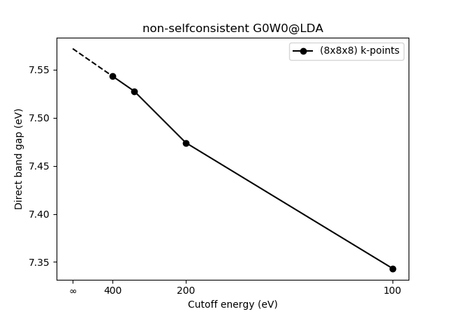
Convergence with respect to cutoff energy and number of k-points
Can we trust the calculated value of the direct bandgap? Not yet. A check for
convergence with respect to the plane wave cutoff energy and number of k
points is necessary. This is done by changing the respective values in the
groundstate calculation and restarting. Script
C_ecut_k_conv_GW.py carries out the calculations and
C_ecut_k_conv_plot_GW.py plots the resulting data. It takes
several hours on a single xeon-8 CPU (8 cores). The resulting figure is
shown below.

A k-point sampling of (8x8x8) seems to give results converged to within 0.005 eV.
The plane wave cutoff is usually converged by employing a \(1/E^{3/2}_{\text{cut}}\) extrapolation.
This can be done with the following script: C_ecut_extrap.py resulting
in a direct band gap of 7.42 eV. The extrapolation is shown in the figure below
Frequency dependence
Next, we should check the quality of the frequency grid used in the
calculation. Two parameters determine how the frequency grid looks.
domega0 and omega2. Read more about these parameters in the tutorial
for the dielectric function Frequency grid.
Running script C_frequency_conv.py calculates the direct band
gap using different frequency grids with domega0 varying from 0.005 to
0.05 and omega2 from 1 to 25. The resulting data is plotted in
C_frequency_conv_plot.py and the figure is shown below.
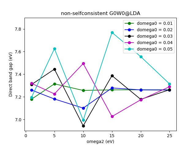
Converged results are obtained for domega0=0.02 and omega2=15, which
is close to the default values.
Final results
A full G0W0 calculation with (8x8x8) k-points and extrapolated to infinite cutoff results in a direct band gap of 7.42 eV. Hence the value of 7.11 eV calculated at first was not converged!
Another method for carrying out the frequency integration is the Plasmon Pole
approximation (PPA). Read more about it here Plasmon Pole Approximation. This is
turned on by setting ppa = True in the G0W0 calculator (see
C_converged_ppa.py). Carrying out a full \(G_0W_0\) calculation with the PPA
using (8x8x8) k-points and extrapolating from calculations at a cutoff of 300
and 400 eV gives a direct band gap of 7.52 eV, which is in very good agreement
with the result for the full frequency integration but the calculation took
only minutes.
Note
Currently PPA does not support Wigner-Seitz supercell truncation and thus the k-point convergence will be lower.
Note
If a calculation is very memory heavy, it is possible to set nblocks
to an integer larger than 1 but less than or equal to the amount of CPU
cores running the calculation. With this, the response function is divided
into blocks and each core gets to store a smaller matrix.
Quasi-particle spectrum of two-dimensional materials
Carrying out a G0W0 calculation of a 2D system follows very much the same recipe
as outlined above for diamond. To avoid having to use a large amount of vacuum in
the out-of-plane direction we advice to use a 2D truncated Coulomb interaction,
which is turned on by setting truncation = '2D'. Additionally it is possible
to add an analytical correction to the q=0 term of the Brillouin zone sampling
by specifying q0_correction=True. This means that a less dense k-point
grid will be necessary to achieve convergence. More information about this
specific method can be found here:
F. A. Rasmussen, P. S. Schmidt, K. T. Winther and K. S. Thygesen
Physical Review B, Vol. 94, 155406 (2016)
How to set up a 2D slab of MoS2 and calculate the band structure can be found in
MoS2_gs_GW.py. The results are not converged but a band gap of 2.57 eV is obtained.
Including vertex corrections
Vertex corrections can be included through the use of a xc kernel known from TDDFT. The vertex corrections can be included in the polarizability and/or the self-energy. It is only physically well justified to include it in both quantities simultaneously. This leads to the \(GW\Gamma\) method. In the \(GW\Gamma\) method, the xc kernel mainly improves the description of short-range correlation which manifests itself in improved absolute band positions. Only including the vertex in the polarizability or the self-energy results in the \(GWP\) and \(GW\Sigma\) method respectively. All three options are available in GPAW. The short-hand notation for the self-energy in the four approximations available is summarized below:
More information can be found here:
P. S. Schmidt, C. E. Patrick, and K. S. Thygesen
Simple vertex correction improves GW band energies of bulk and two-dimensional crystals
To appear in Physical Review B.
Note
Including vertex corrections is currently not possible for spin-polarized systems.
A \(GW\Gamma\) calculation requires that two additional keywords are specified in the GW calculator:
Which kernel to use:
xc='rALDA',xc='rAPBE'etc..How to apply the kernel:
fxc_mode = 'GWG',fxc_mode='GWP'orfxc_mode='GWS'.
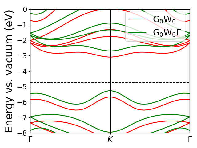
Carrying on from the ground state calculation in MoS2_gs_GW.py, a \(GW\Gamma\) calculation can be done with the following script: MoS2_GWG.py.
The \(GW\) and \(GW\Gamma\) band structures can be visualized with the MoS2_bs_plot.py script resulting in the figure below. Here, the effect of the vertex is to shift the bands upwards by around 0.5 eV whilst leaving the band gap almost unaffected.
Note
When carrying out a \(G_0W_0\Gamma\) calculation by specifying the 3 keywords above, the do_GW_too = True option allows for a simultaneous \(G_0W_0\) calculation. This is faster than doing two seperate calculations as \(\chi_0\) only needs to be calculated once, but the memory requirement is twice that of a single \(G_0W_0\) calculation. The \(G_0W_0\Gamma\) results will by default be stored in g0w0_results.pckl and the \(G_0W_0\) results in g0w0_results_GW.pckl. The results of both calculations will be printed in the output .txt file.