Circular dichroism with real-time TDDFT

In this tutorial, we calculate the rotatory strength spectrum of (R)-methyloxirane molecule.

The equations underlying the implementation are described in Ref. [1].

LCAO mode

In this example, we use real-time TDDFT LCAO mode. We recall that the LCAO calculations are sensitive to the used basis sets, and we also demonstrate the construction of augmented basis sets.

We augment the default dzp basis sets with numerical Gaussian-type orbitals (NGTOs):

from gpaw.lcao.generate_ngto_augmented import \
    create_GTO_dictionary as GTO, generate_nao_ngto_basis

gtos_atom = {'H': [GTO('s', 0.02974),
                   GTO('p', 0.14100)],
             'C': [GTO('s', 0.04690),
                   GTO('p', 0.04041),
                   GTO('d', 0.15100)],
             'O': [GTO('s', 0.07896),
                   GTO('p', 0.06856),
                   GTO('d', 0.33200)],
             }

for atom in ['H', 'C', 'O']:
    generate_nao_ngto_basis(atom, xc='PBE', name='aug',
                            nao='dzp', gtos=gtos_atom[atom])

Here, the Gaussian parameters correspond to diffuse functions in aug-cc-pvdz basis sets as obtained from Basis Set Exchange.

Let’s do the ground-state calculation (note the basis keyword):

from ase.io import read
from gpaw import setup_paths
from gpaw import GPAW

# Insert the path to the created basis set
setup_paths.insert(0, '.')

atoms = read('r-methyloxirane.xyz')
atoms.center(vacuum=6.0)

calc = GPAW(mode='lcao',
            basis='aug.dzp',
            h=0.3,
            xc='PBE',
            nbands=16,
            poissonsolver={
                'name': 'MomentCorrectionPoissonSolver',
                'poissonsolver': 'fast',
                'moment_corrections': 1 + 3 + 5},
            convergence={'density': 1e-12},
            txt='gs.out',
            symmetry={'point_group': False})
atoms.calc = calc
atoms.get_potential_energy()
calc.write('gs.gpw', mode='all')

Then, we carry the time propagation as usual in real-time TDDFT LCAO mode, but we attach MagneticMomentWriter to record the time-dependent magnetic moment. In this script, we wrap the time propagation code inside main() function to make the same script reusable with different kick directions:

from gpaw import setup_paths
from gpaw.lcaotddft import LCAOTDDFT
from gpaw.lcaotddft.dipolemomentwriter import DipoleMomentWriter
from gpaw.lcaotddft.magneticmomentwriter import MagneticMomentWriter

# Insert the path to the created basis set
setup_paths.insert(0, '.')


def main(kick):
    kick_strength = [0., 0., 0.]
    kick_strength['xyz'.index(kick)] = 1e-5

    td_calc = LCAOTDDFT('gs.gpw', txt=f'td-{kick}.out')

    DipoleMomentWriter(td_calc, f'dm-{kick}.dat')
    MagneticMomentWriter(td_calc, f'mm-{kick}.dat')

    td_calc.absorption_kick(kick_strength)
    td_calc.propagate(10, 2000)

    td_calc.write(f'td-{kick}.gpw', mode='all')


if __name__ == '__main__':
    import argparse
    parser = argparse.ArgumentParser()
    parser.add_argument('--kick', default='x')
    kwargs = vars(parser.parse_args())
    main(**kwargs)

After repeating the calculation for kicks in x, y, and z directions, we calculate the rotatory strength spectrum from the magnetic moments:

from gpaw.tddft.spectrum import rotatory_strength_spectrum

rotatory_strength_spectrum(['mm-x.dat', 'mm-y.dat', 'mm-z.dat'],
                           'rot_spec.dat',
                           folding='Gauss', width=0.2,
                           e_min=0.0, e_max=10.0, delta_e=0.01)

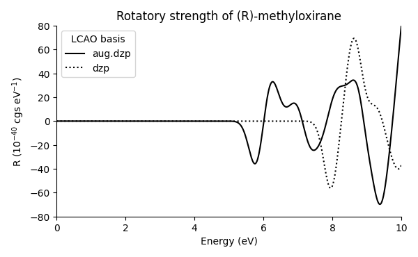
Comparing the resulting spectrum to one calculated with plain dzp basis sets shows the importance of augmented basis sets:

FD mode

In this example, we use real-time TDDFT FD mode.

Let’s do the ground-state calculation (note that FD mode typically requires larger vacuum and smaller grid spacing than LCAO mode; convergence with respect to these parameters need to be checked for both modes separately):

from ase.io import read
from gpaw import GPAW

atoms = read('r-methyloxirane.xyz')
atoms.center(vacuum=8.0)

calc = GPAW(mode='fd',
            h=0.2,
            xc='PBE',
            nbands=16,
            poissonsolver={
                'name': 'MomentCorrectionPoissonSolver',
                'poissonsolver': 'fast',
                'moment_corrections': 1 + 3 + 5},
            convergence={'density': 1e-12},
            txt='gs.out',
            symmetry={'point_group': False})
atoms.calc = calc
atoms.get_potential_energy()
calc.write('gs.gpw', mode='all')

Then, similarly to LCAO mode, we carry the time propagation as usual but attach MagneticMomentWriter to record the time-dependent magnetic moment (note the tolerance parameter for the iterative solver; smaller values might be required when signal is weak):

from gpaw.tddft import TDDFT, DipoleMomentWriter, MagneticMomentWriter


def main(kick):
    kick_strength = [0., 0., 0.]
    kick_strength['xyz'.index(kick)] = 1e-5

    td_calc = TDDFT('gs.gpw',
                    solver=dict(name='CSCG', tolerance=1e-8),
                    txt=f'td-{kick}.out')

    DipoleMomentWriter(td_calc, f'dm-{kick}.dat')
    MagneticMomentWriter(td_calc, f'mm-{kick}.dat')

    td_calc.absorption_kick(kick_strength)
    td_calc.propagate(10, 2000)

    td_calc.write(f'td-{kick}.gpw', mode='all')


if __name__ == '__main__':
    import argparse
    parser = argparse.ArgumentParser()
    parser.add_argument('--kick', default='x')
    kwargs = vars(parser.parse_args())
    main(**kwargs)

After repeating the calculation for kicks in x, y, and z directions, we calculate the rotatory strength spectrum from the magnetic moments:

from gpaw.tddft.spectrum import rotatory_strength_spectrum

rotatory_strength_spectrum(['mm-x.dat', 'mm-y.dat', 'mm-z.dat'],
                           'rot_spec.dat',
                           folding='Gauss', width=0.2,
                           e_min=0.0, e_max=10.0, delta_e=0.01)

The resulting spectrum:

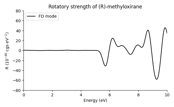
The spectrum compares well with the one obtained with LCAO mode and augmented basis sets.

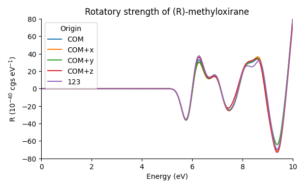
Origin dependence

The circular dichroism spectra obtained with the present implementation depend on the choice of origin. See the documentation of MagneticMomentWriter for parameters controlling the origin location.

The magnetic moment data can be written at multiple different origins during a single propagation as demonstrated in this script:

from gpaw import setup_paths
from gpaw.lcaotddft import LCAOTDDFT
from gpaw.lcaotddft.dipolemomentwriter import DipoleMomentWriter
from gpaw.lcaotddft.magneticmomentwriter import MagneticMomentWriter

# Insert the path to the created basis set
setup_paths.insert(0, '.')


def main(kick):
    kick_strength = [0., 0., 0.]
    kick_strength['xyz'.index(kick)] = 1e-5

    td_calc = LCAOTDDFT('gs.gpw', txt=f'td-{kick}.out')

    DipoleMomentWriter(td_calc, f'dm-{kick}.dat')

    # Origin: center of mass
    MagneticMomentWriter(td_calc, f'mm-COM-{kick}.dat',
                         origin='COM')

    # Origin: center of mass + 5 Å shift
    for shift_axis in 'xyz':
        origin_shift = [0, 0, 0]
        origin_shift['xyz'.index(shift_axis)] = 5
        MagneticMomentWriter(td_calc, f'mm-COM+{shift_axis}-{kick}.dat',
                             origin='COM', origin_shift=origin_shift)

    # Origin: arbitrary coordinate
    MagneticMomentWriter(td_calc, f'mm-123-{kick}.dat',
                         origin='zero', origin_shift=[1, 2, 3])

    td_calc.absorption_kick(kick_strength)
    td_calc.propagate(10, 2000)

    td_calc.write(f'td-{kick}.gpw', mode='all')


if __name__ == '__main__':
    import argparse
    parser = argparse.ArgumentParser()
    parser.add_argument('--kick', default='x')
    kwargs = vars(parser.parse_args())
    main(**kwargs)

The resulting spectra:

References

[1]

E. Makkonen, T. P. Rossi, A. H. Larsen, O. Lopez-Acevedo, P. Rinke, M. Kuisma, and X. Chen,

Real-time time-dependent density functional theory implementation of electronic circular dichroism applied to nanoscale metal-organic clusters

J. Chem. Phys. 154, 114102 (2021)