The Bethe-Salpeter equation and Excitons
For a brief introduction to the Bethe-Salpeter equation and the details of its implementation in GPAW, see Bethe-Salpeter Equation - Theory.
Absorption spectrum of bulk silicon
We start by calculating the ground state density and diagonalizing the
resulting Hamiltonian. Below we will set up the Bethe-Salpeter Hamiltonian
in a basis of the 4 valence bands and 4 conduction bands. However, the
screened interaction that enters the Hamiltonian needs to be converged with
respect the number of unoccupied bands. The calculaton is erfored with the
following script gs_Si.py. It takes a few minutes on a single
CPU. The last line in the script creates a .gpw file which contains all the
informations of the system, including the wavefunctions.
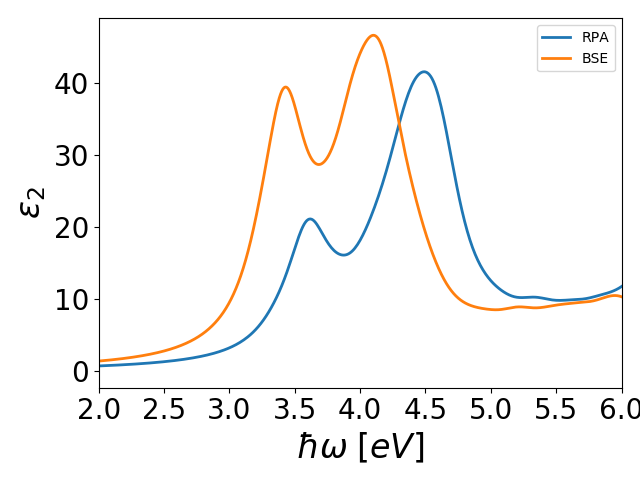
Next we calculate the dynamical dielectric function using the
Bethe-Salpeter equation. The imaginary part is proportional to the
absorption spectrum. The calculation can be done with the script
eps_Si.py, which also calculates the dielectric function within
the Random Phase Approximation (see Linear dielectric response of an extended system). It takes about ~12
hours on a single CPU but parallelizes very well. Note the .csv output
files that contains the spectre. The script also generates a .dat file
that contains the eigenvalues of the BSE eigenvalues for easy application.
The spectrum essentially consists of a number of peaks centered on the
eigenvalues. It can be plottet with plot_Si.py and the result
is shown below
The parameters that need to be converged in the calculation are the
k-points in the initial ground state calculation. In addition the
following keywords in the BSE object should be converged: the plane wave
cutoff ecut, the numbers of bands used to calculate the screened
interaction nbands, the list of valence bands valence_bands and the
list of conduction bands conduction_bands included in the Hamiltonian.
It is also possible to provide an array gw_skn, with GW eigenvalues to
be used in the non-interacting part of th Hamiltonian. Here, the indices
denote spin, k-points and bands, which has to match the spin, k-point
sampling and the number of specified valence and conduction bands in the
ground state calculation.
Excitons in monolayer MoS2 with Spin-orbit Coupling
Spectrum from the Bethe-Salpeter equation
The screening plays a fundamental role in the Bethe-Salpeter equation and for 2D systems the screening requires a special treatment. In particular we use a truncated Coulomb interaction inorder to decouple the screening between periodic images. We refer to Ref. [1] for details on the truncated Coulomb interaction in GPAW. As before, we calculate the ground state of \(MoS_2\) with the script gs_MoS2.py, which takes a few minutes. Note the large density of k-points, which are required to converge the BSE spectrum of two-dimensional systems.
The macroscopic dielectric function is calculated as an average of the microscopic screening over the unit cell. Clearly, for a 2D system this will depend on the unit cell size in the direction orthogonal to the slab and in the converged limit the dielectric function becomes unity. Instead we may calculate the longitudinal part of 2D polarizability which is independent of unit cell size. This is done in RPA as well as BSE with the scripts pol_MoS2.py, which takes ~20 hours on 16 CPUs. Note that the BSE polarizability is calculated with and without Coulomb truncation for comparison. In both case spin-orbit coupling is included through the spinors keyword. We refer to Ref. [2] for details on the spin-orbit implementation. The results can be plottet with plot_MoS2.py and is shown below.
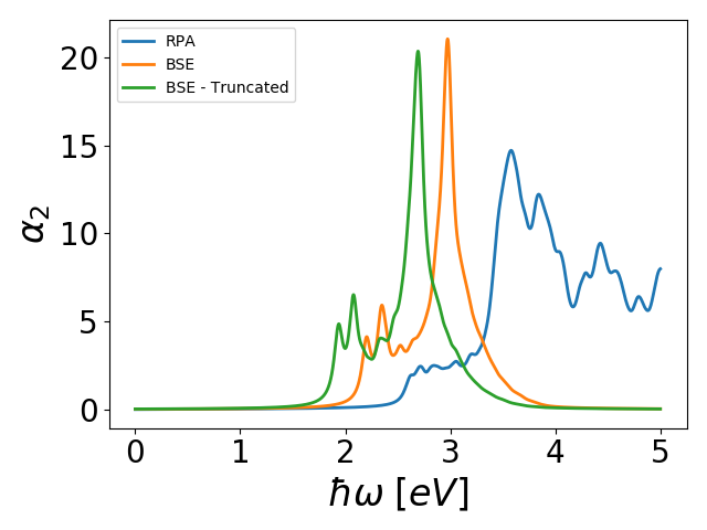
The excitonic effects are much stronger than in the case of Si due to the reduced screening in 2D. In particular, we can identify a distinct spin-orbit split exciton well below the band edge. Note that without Coulomb truncation, the BSE spectrum is shifted upward in energy due the screening of electron-hole interactions from periodic images.
2D screening with and without Coulomb truncation
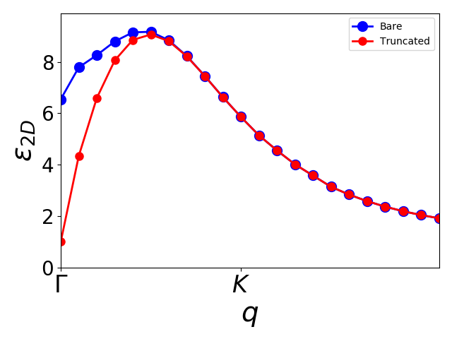
To see the effect of the Coulomb truncation, which eliminates the screening from layers in periodic images, we will now calculate the dielectric constant evaluated at the center of the layer \(z_0\) and averaged in the plane. This is accomplished with
The script get_2d_eps.py carries out this calculations with and without Coulomb truncation and the result is shown below plot_2d_eps.py. Note that the truncated screening is bound to become one at \(\Gamma\) due to the different behavior of Coulomb interaction (in \(q\)-space) in 2D systems. For small values of \(q\) the screening is linear, which makes convergence tricky in standard Brillouin zone sampling schemes. Since the \(\Gamma\)-point is always sampled, the screening is typically underestimated and the exciton binding energy is too high at finite \(k\)-point samplings.
Mott-Wannier model for excitons in 2D materials
In 3D materials the Mott-Wannier model of excitons has been highly succesful and simply regards the exciton as a “hydrogen atom” with bindings energies that has been rescaled by the exciton effective mass and dielectric screening. Thus in atomic units the binding energy is
where \(\mu^{-1}=m_v^{-1}+m_c^{-1}\) and \(m_v\) and \(m_c\) are the masses of valence and conduction electrons respectively. The 3D expression relies on the fact that the screening is local in real space and thus approximately independent of \(q\). This is clearly not the case in 2D where we always have
for small \(q\). It is thus expected that the hydrogenic binding energy in 2D becomes renormalized by the slope \(\alpha\) in addition to the effective mass. Indeed in Ref. [3] it was shown that the binding energy in 2D can be approximated by
From the band structure of MoS2 it is straigtforward to obtain \(\mu=0.27\) and all we need now is \(\alpha\). In principle we could read of the slope from the figure above, but there is a more direct an accurate way to do it. As it turns out, the slope is needed for any calculation of the response function in the optical limit and it is simply obtained with the script alpha_MoS2.py. This runs on a single CPU in a minute or so. It should produce a value of \(\alpha=5.27\) Å. Transforming to atomic units and inserting into the formula above yields
which is in good agreement with the BSE computation above