Introduction to GPAW internals

This guide will contain graphs showing the relationship between objects that build up a DFT calculation engine.

Hint

Here is a simple graph showing the relations between the classes A, B and C:

Here, the object of type A has an attribute a of type int and an attribute b of type B or C, where C inherits from B.

DFT components

The components needed for a DFT calculation are created by a “builder” that can be made with the builder() function, an ASE ase.Atoms object and some input parameters:

>>> from ase import Atoms
>>> atoms = Atoms('Li', cell=[2, 2, 2], pbc=True)
>>> from gpaw.new.builder import builder
>>> params = {'mode': 'pw', 'kpts': (5, 5, 5), 'txt': None}
>>> b = builder(atoms, params)

As seen in the figure above, there are builders for each of the modes: PW, FD and LCAO (builders for TB and ATOM modes are not shown).

The InputParameters object takes care of user parameters:

• checks for errors

• does normalization

• handles backwards compatibility and deprecation warnings

Normally, you will not need to create a DFT-components builder yourself. It will happen automatically when you create a DFT-calculation object like this:

>>> from gpaw.new.calculation import DFTCalculation
>>> calculation = DFTCalculation.from_parameters(atoms, params)

or when you create an ASE-calculator interface:

>>> from gpaw.new.ase_interface import GPAW
>>> atoms.calc = GPAW(**params)

Full picture

The ase.Atoms object has an gpaw.new.ase_interface.ASECalculator object attached created with the gpaw.new.ase_interface.GPAW() function:

>>> atoms = Atoms('H2',
...               positions=[(0, 0, 0), (0, 0, 0.75)],
...               cell=[2, 2, 3],
...               pbc=True)
>>> atoms.calc = GPAW(mode='pw', txt='h2.txt')
>>> atoms.calc
ASECalculator(mode: {'name': 'pw'}, txt: 'h2.txt')

The atoms.calc object manages a gpaw.new.calculation.DFTCalculation object that does the actual work. When we do this:

>>> e = atoms.get_potential_energy()

the gpaw.new.ase_interface.ASECalculator.get_potential_energy() method gets called (atoms.calc.get_potential_energy(atoms)) and the following will happen:

• create gpaw.new.calculation.DFTCalculation object if not already done

• update positions/unit cell if they have changed

• start SCF loop and converge if needed

• calculate energy

• store a copy of the atoms

Do-it-yourself example

Let’s try to build a DFT calculation without any of the shortcuts (gpaw.new.builder.builder(), gpaw.new.ase_interface.GPAW() or gpaw.new.calculation.DFTCalculation.from_parameters()).

So, instead of simple three-line example above where we calculate the energy of an H2 molecule, we do it the hard way:

from ase import Atoms
from ase.units import Bohr
from gpaw.setup import Setups
from gpaw.new.xc import XCFunctional
from gpaw.new.density import Density
from gpaw.core import UniformGrid
from gpaw.new.basis import create_basis
from gpaw.new.symmetry import create_symmetries_object
from gpaw.new.brillouin import BZPoints
from gpaw.core.atom_arrays import AtomDistribution
from gpaw.mpi import world

atoms = Atoms('H2',
              positions=[(0, 0, 0), (0, 0, 0.75)],
              cell=[2, 2, 3],
              pbc=True)

xc = XCFunctional('LDA')
setups = Setups([1, 1], {}, {}, xc)
grid = UniformGrid(cell=atoms.cell / Bohr,
                   size=[10, 10, 15],
                   pbc=[True, True, True])
symmetries = create_symmetries_object(atoms)
ibz = symmetries.reduce(BZPoints([[0, 0, 0]]))
basis = create_basis(
    ibz,
    nspins=1,
    pbc_c=atoms.pbc,
    grid=grid,
    setups=setups,
    dtype=float,
    fracpos_ac=atoms.get_scaled_positions())
nct_R = grid.zeros()
atomdist = AtomDistribution([0, 0], world)
density = Density.from_superposition(grid, nct_R, atomdist, setups, basis)
pot_calc = ...
potential = ...
wfs = ...
ibzwfs = ...
state = ...
scf_loop = ...
for _ in scf_loop.iterate(state, pot_calc):
    ...

DFT-calculation object

An instance of the gpaw.new.calculation.DFTCalculation class has the following attributes:

state	gpaw.new.calculation.DFTState
scf_loop	gpaw.new.scf.SCFLoop
pot_calc	gpaw.new.pot_calc.PotentialCalculator

and a the gpaw.new.calculation.DFTState object has these attributes:

density	gpaw.new.density.Density
ibzwfs	gpaw.new.ibzwfs.IBZWaveFunctions
potential	gpaw.new.potential.Potential

Naming convention for arrays

Commonly used indices:

index	description
a	Atom number
c	Unit cell axis-index (0, 1, 2)
v	xyz-index (0, 1, 2)
K	BZ k-point index
k	IBZ k-point index
q	IBZ k-point index (local, i.e. it starts at 0 on each processor)
s	Spin index (\(\sigma\))
s	Symmetry index
u	Combined spin and k-point index (local)
R	Three indices into the coarse 3D grid
r	Three indices into the fine 3D grid
G	Index of plane-wave coefficient (wave function expansion, ecut)
g	Index of plane-wave coefficient (densities, 2 * ecut)
h	Index of plane-wave coefficient (compensation charges, 8 * ecut)
X	R or G
x	r, g or h
x	Zero or more extra dimensions
M	LCAO orbital index (\(\mu\))
n	Band number
n	Principal quantum number
l	Angular momentum quantum number (s, p, d, …)
m	Magnetic quantum number (0, 1, …, 2*`ell` - 1)
L	l and m (L = l**2 + m)
j	Valence orbital number (n and l)
i	Valence orbital number (n, l and m)
q	j1 and j2 pair
p	i1 and i2 pair
r	CPU-rank

Examples:

density.D_asii	\(D_{\sigma,i_1,i_2}^a\)	AtomArrays
density.nt_sR	\(\tilde{n}_\sigma(\mathbf{r})\)	UniformGridFunctions
ibzwfs.wfs_qs[q][s].P_ain	\(P_{\sigma \mathbf{k} in}^a\)	AtomArrays
ibzwfs.wfs_qs[q][s].psit_nX	\(\tilde{\psi}_{\sigma \mathbf{k} n}(\mathbf{r})\)	UniformGridFunctions | PlaneWaveExpansions
ibzwfs.wfs_qs[q][s].pt_aX	\(\tilde{p}_{\sigma \mathbf{k} i}^a(\mathbf{r}-\mathbf{R}^a)\)	AtomCenteredFunctions

Domain descriptors

GPAW has two different container types for storing one or more functions in a unit cell (wave functions, electron densities, …):

• PlaneWaveExpansions

• UniformGridFunctions

Uniform grids

A uniform grid can be created with the UniformGrid class:

>>> import numpy as np
>>> from gpaw.core import UniformGrid
>>> a = 4.0
>>> n = 20
>>> grid = UniformGrid(cell=a * np.eye(3),
...                    size=(n, n, n))

Given a UniformGrid object, one can create UniformGridFunctions objects like this

>>> func_R = grid.empty()
>>> func_R.data.shape
(20, 20, 20)
>>> func_R.data[:] = 1.0
>>> grid.zeros((3, 2)).data.shape
(3, 2, 20, 20, 20)

Here are the methods of the UniformGrid class:

size()	Size of uniform grid.
global_shape()	Actual size of uniform grid.
phase_factors_cd()	…
new()	Create new uniform grid description.
empty()	Create new UniformGridFunctions object.
blocks()	Yield views of blocks of data.
xyz()	Create array of (x, y, z) coordinates.
atom_centered_functions()	Create UniformGridAtomCenteredFunctions object.
transformer()	Create transformer from one grid to another.
eikr()	Plane wave.
from_cell_and_grid_spacing()	Create UniformGrid from grid-spacing.
fft_plans()	Create FFTW-plans.
ranks_from_fractional_positions()	…
ecut_max()	…

and the UniformGridFunctions class:

new()	Create new UniforGridFunctions object of same kind.
xy()	Extract x, y values along line.
scatter_from()	Scatter data from rank-0 to all ranks.
gather()	Gather data from all ranks to rank-0.
fft()	Do FFT.
norm2()	Calculate integral over cell of absolute value squared.
integrate()	Integral of self or self times cc(other).
to_pbc_grid()	Convert to UniformGrud with pbc=(True, True, True).
multiply_by_eikr()	Multiply by \(exp(ik.r)\).
interpolate()	Interpolate to finer grid.
fft_restrict()	Restrict to coarser grid.
abs_square()	Add weighted absolute square of data to output array.
symmetrize()	Make data symmetric.
randomize()	Insert random numbers between -0.5 and 0.5 into data.
moment()	Calculate moment of data.
scaled()	Create new scaled UniformGridFunctions object.

Plane waves

A set of plane-waves are characterized by a cutoff energy and a uniform grid:

>>> from gpaw.core import PlaneWaves
>>> pw = PlaneWaves(ecut=100, cell=grid.cell)
>>> func_G = pw.empty()
>>> func_R.fft(out=func_G)
PlaneWaveExpansions(pw=PlaneWaves(ecut=100 <coefs=1536/1536>, cell=[4.0, 4.0, 4.0], pbc=[True, True, True], comm=0/1, dtype=float64), dims=())
>>> G = pw.reciprocal_vectors()
>>> G.shape
(1536, 3)
>>> G[0]
array([0., 0., 0.])
>>> func_G.data[0]
(1+0j)
>>> func_G.ifft(out=func_R)
UniformGridFunctions(grid=UniformGrid(size=[20, 20, 20], cell=[4.0, 4.0, 4.0], pbc=[True, True, True], comm=0/1, dtype=float64), dims=())
>>> round(func_R.data[0, 0, 0], 15)
1.0

Here are the methods of the PlaneWaves class:

itemsize()	int([x]) -> integer
global_shape()	Tuple with one element: number of plane waves.
reciprocal_vectors()	Returns reciprocal lattice vectors, G + k, in xyz coordinates.
kinetic_energies()	Kinetic energy of plane waves.
empty()	Create new PlaneWaveExpanions object.
new()	Create new plane-wave expansion description.
indices()	Return indices into FFT-grid.
cut()	Cut out G-vectors with (G+k)^2/2<E_kin.
paste()	Paste G-vectors with (G+k)^2/2<E_kin into 3-D FFT grid and
map_indices()	Map from one (distributed) set of plane waves to smaller global set.
atom_centered_functions()	Create PlaneWaveAtomCenteredFunctions object.

and the PlaneWaveExpansions class:

new()	Create new PlaneWaveExpansions object of same kind.
copy()	Create a copy (surprise!).
matrix()	Matrix view of data.
ifft()	Do inverse FFT(s) to uniform grid(s).
interpolate()	…
gather()	Gather coefficients on master.
gather_all()	Gather coefficients from self[r] on rank r.
scatter_from()	Scatter data from rank-0 to all ranks.
scatter_from_all()	Scatter all coefficients from rank r to self on other cores.
integrate()	Integral of self or self time cc(other).
norm2()	Calculate integral over cell.
abs_square()	Add weighted absolute square of self to output array.
to_pbc_grid()	…
randomize()	Insert random numbers between -0.5 and 0.5 into data.
moment()	…
morph()	…

Atoms-arrays

Block boundary conditions

…

Matrix elements

>>> psit_nG = pw.zeros(5)
>>> def T(psit_nG):
...     """Kinetic energy operator."""
...     out = psit_nG.new()
...     out.data[:] = psit_nG.desc.ekin_G * psit_nG.data
...     return out
>>> H_nn = psit_nG.matrix_elements(psit_nG, function=T)

Same as:

>>> Tpsit_nG = T(psit_nG)
>>> psit_nG.matrix_elements(Tpsit_nG, symmetric=True)
Matrix(float64: 5x5)

but faster.

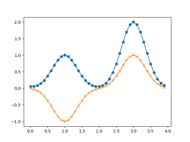
Atom-centered functions

# creates: acf_example.png
import numpy as np
import matplotlib.pyplot as plt
from gpaw.core import UniformGrid


alpha = 4.0
rcut = 2.0
l = 0
gauss = (l, rcut, lambda r: (4 * np.pi)**0.5 * np.exp(-alpha * r**2))
grid = UniformGrid(cell=[4.0, 2.0, 2.0], size=[40, 20, 20])
pos = [[0.25, 0.5, 0.5], [0.75, 0.5, 0.5]]
acf_aR = grid.atom_centered_functions([[gauss], [gauss]], pos)
coef_as = acf_aR.empty(dims=(2,))
coef_as[0] = [[1], [-1]]
coef_as[1] = [[2], [1]]
print(coef_as.data, coef_as[0])
f_sR = grid.zeros(2)
acf_aR.add_to(f_sR, coef_as)
x = grid.xyz()[:, 10, 10, 0]
y1, y2 = f_sR.data[:, :, 10, 10]
ax = plt.subplot(1, 1, 1)
ax.plot(x, y1, 'o-')
ax.plot(x, y2, 'x-')
# plt.show()
plt.savefig('acf_example.png')

Matrix object

Here are the methods of the Matrix class:

new()	Create new matrix of same shape and dtype.
copy()	Create a copy.
multiply()	BLAS matrix-multiplication with other matrix.
redist()	Redistribute to other BLACS layout.
gather()	Gather the Matrix on the root rank.
inv()	Inplace inversion.
invcholesky()	In-place inverse of Cholesky decomposition.
eigh()	Calculate eigenvectors and eigenvalues.
eighg()	Solve generalized eigenvalue problem.
complex_conjugate()	Inplace complex conjugation.
add_hermitian_conjugate()	Add hermitian conjugate to myself.
tril2full()	Fill in upper triangle from lower triangle.
add_to_diagonal()	Add list of numbers or single number to diagonal of matrix.
to_cpu()	…

A simple example that we can run with MPI on 4 cores:

from gpaw.core.matrix import Matrix
from gpaw.mpi import world
a = Matrix(5, 5, dist=(world, 2, 2, 2))
a.data[:] = world.rank
print(world.rank, a.data.shape)

Here, we have created a 5x5 Matrix of floats distributed on a 2x2 BLACS grid with a block size of 2 and we then print the shapes of the ndarrays, which looks like this (in random order):

1 (2, 3)
2 (3, 2)
3 (2, 2)
0 (3, 3)

Let’s create a new matrix b and redistribute from a to b:

b = a.new(dist=(None, 1, 1, None))
a.redist(b)
if world.rank == 0:
    print(b.array)

This will output:

[[ 0.  0.  2.  2.  0.]
 [ 0.  0.  2.  2.  0.]
 [ 1.  1.  3.  3.  1.]
 [ 1.  1.  3.  3.  1.]
 [ 0.  0.  2.  2.  0.]]

Matrix-matrix multiplication works like this:

c = a.multiply(a, opb='T')

API

Core

class gpaw.core.UniformGrid(*, cell, size, pbc=(True, True, True), kpt=None, comm=<gpaw.mpi._Communicator object>, decomp=None, dtype=None)

Description of 3D uniform grid.

Parameters:

• cell (ArrayLike1D | ArrayLike2D) – Unit cell given as three floats (orthorhombic grid), six floats (three lengths and the angles in degrees) or a 3x3 matrix.

• size (ArrayLike1D) – Number of grid points along axes.

• pbc – Periodic boundary conditions flag(s).

• comm (MPIComm) – Communicator for domain-decomposition.

• kpt (Vector) – K-point for Block-boundary conditions specified in units of the reciprocal cell.

• decomp (Sequence[Sequence[int]]) – Decomposition of the domain.

• dtype – Data-type (float or complex).

atom_centered_functions(functions, positions, *, atomdist=None, integral=None, cut=False, xp=None)

Create UniformGridAtomCenteredFunctions object.

blocks(data)

Yield views of blocks of data.

ecut_max()

eikr(kpt_c=None)

Plane wave.

\[e^{i\mathbf{k}\cdot \mathbf{r}}\]

Parameters:

kpt_c (Optional[Union[Sequence[float], ndarray]]) – k-point in units of the reciprocal cell. Defaults to the UniformGrid objects own k-point.

empty(dims=(), comm=<gpaw.mpi._Communicator object>, xp=<module 'numpy' from '/tmp/gpaw-docs/venv/lib/python3.10/site-packages/numpy/__init__.py'>)

Create new UniformGridFunctions object.

Parameters:

• dims (int | tuple[int, ...]) – Extra dimensions.

• comm (Any) – Distribute dimensions along this communicator.

fft_plans(flags=0, xp=<module 'numpy' from '/tmp/gpaw-docs/venv/lib/python3.10/site-packages/numpy/__init__.py'>)

Create FFTW-plans.

classmethod from_cell_and_grid_spacing(cell, grid_spacing, pbc=(True, True, True), kpt=None, comm=<gpaw.mpi._Communicator object>, dtype=None)

Create UniformGrid from grid-spacing.

global_shape()

Actual size of uniform grid.

new(size=None, pbc=None, kpt=None, comm='inherit', decomp=None, dtype=None)

Create new uniform grid description.

property phase_factors_cd

ranks_from_fractional_positions(fracpos_ac)

property size

Size of uniform grid.

transformer(other, stencil_range=3)

Create transformer from one grid to another.

(for interpolation and restriction).

xyz()

Create array of (x, y, z) coordinates.

class gpaw.core.PlaneWaves(*, ecut, cell, kpt=None, comm=<gpaw.mpi._Communicator object>, dtype=None)

Description of plane-wave basis.

Parameters:

• ecut (float) – Cutoff energy for kinetic energy of plane waves.

• cell (ArrayLike1D | ArrayLike2D) – Unit cell given as three floats (orthorhombic grid), six floats (three lengths and the angles in degrees) or a 3x3 matrix.

• comm (MPIComm) – Communicator for distribution of plane-waves.

• kpt (Vector) – K-point for Block-boundary conditions specified in units of the reciprocal cell.

• dtype – Data-type (float or complex).

atom_centered_functions(functions, positions, *, atomdist=None, integral=None, cut=False, xp=None)

Create PlaneWaveAtomCenteredFunctions object.

cut(array_Q)

Cut out G-vectors with (G+k)^2/2<E_kin.

empty(dims=(), comm=<gpaw.mpi._Communicator object>, xp=None)

Create new PlaneWaveExpanions object.

Parameters:

• dims (int | tuple[int, ...]) – Extra dimensions.

• comm (Any) – Distribute dimensions along this communicator.

global_shape()

Tuple with one element: number of plane waves.

indices(shape)

Return indices into FFT-grid.

itemsize: int = 16

kinetic_energies()

Kinetic energy of plane waves.

\[|\mathbf{G}+\mathbf{k}|^{2} / 2\]

map_indices(other)

Map from one (distributed) set of plane waves to smaller global set.

Say we have 9 G-vector on two cores:

5 3 4             . 3 4           0 . .
2 0 1 -> rank=0:  2 0 1  rank=1:  . . .
8 6 7             . . .           3 1 2

and we want a mapping to these 5 G-vectors:

  3
2 0 1
  4

On rank=0: the return values are:

[0, 1, 2, 3], [[0, 1, 2, 3], [4]]

and for rank=1:

[1], [[0, 1, 2, 3], [4]]

new(*, ecut=None, kpt=None, comm='inherit')

Create new plane-wave expansion description.

paste(coef_G, array_Q)

Paste G-vectors with (G+k)^2/2<E_kin into 3-D FFT grid and zero-pad.

reciprocal_vectors()

Returns reciprocal lattice vectors, G + k, in xyz coordinates.

class gpaw.core.atom_centered_functions.AtomCenteredFunctions(functions, fracpos_ac, atomdist=None, xp=None)

add_to(functions, coefs=1.0)

Add atom-centered functions multiplied by coefs to functions.

property atomdist

derivative(functions, out=None)

Calculate derivatives of integrals with respect to atom positions.

empty(dims=(), comm=<gpaw.mpi._Communicator object>)

Create AtomsArray for coefficients.

integrate(functions, out=None)

Calculate integrals of atom-centered functions multiplied by functions.

property layout

move(fracpos_ac, atomdist)

Move atoms to new positions.

stress_tensor_contribution(a, c=1.0)

class gpaw.core.uniform_grid.UniformGridFunctions(grid, dims=(), comm=<gpaw.mpi._Communicator object>, data=None, xp=None)

Object for storing function(s) on a uniform grid.

Parameters:

• grid (UniformGrid) – Description of uniform grid.

• dims (int | tuple[int, ...]) – Extra dimensions.

• comm (MPIComm) – Distribute dimensions along this communicator.

• data (np.ndarray) – Data array for storage.

abs_square(weights, out=None)

Add weighted absolute square of data to output array.

fft(plan=None, pw=None, out=None)

Do FFT.

\[\int d\mathbf{r} e^{i\mathbf{G}\cdot \mathbf{r}} f(\mathbf{r})\]

fft_restrict(plan1=None, plan2=None, grid=None, out=None)

Restrict to coarser grid.

Parameters:

• plan1 (Optional[FFTPlans]) – Plan for FFT.

• plan2 (Optional[FFTPlans]) – Plan for inverse FFT.

• grid (Optional[UniformGrid]) – Target grid.

• out (Optional[UniformGridFunctions]) – Target UniformGridFunctions object.

gather(out=None, broadcast=False)

Gather data from all ranks to rank-0.

integrate(other=None)

Integral of self or self times cc(other).

interpolate(plan1=None, plan2=None, grid=None, out=None)

Interpolate to finer grid.

Parameters:

• plan1 (Optional[FFTPlans]) – Plan for FFT (course grid).

• plan2 (Optional[FFTPlans]) – Plan for inverse FFT (fine grid).

• grid (Optional[UniformGrid]) – Target grid.

• out (Optional[UniformGridFunctions]) – Target UniformGridFunctions object.

moment(center_v=None)

Calculate moment of data.

multiply_by_eikr(kpt_c=None)

Multiply by \(exp(ik.r)\).

new(data=None)

Create new UniforGridFunctions object of same kind.

Parameters:

data – Array to use for storage.

norm2()

Calculate integral over cell of absolute value squared.

\[\int |a(\mathbf{r})|^{2} d\mathbf{r}\]

randomize()

Insert random numbers between -0.5 and 0.5 into data.

scaled(s, v=1.0)

Create new scaled UniformGridFunctions object.

Unit cell axes are multiplied by \(s\) and data by \(v\).

scatter_from(data=None)

Scatter data from rank-0 to all ranks.

symmetrize(rotation_scc, translation_sc)

Make data symmetric.

to_pbc_grid()

Convert to UniformGrud with pbc=(True, True, True).

xy(*axes)

Extract x, y values along line.

Useful for plotting:

x, y = grid.xy(0, ..., 0)
plt.plot(x, y)

class gpaw.core.arrays.DistributedArrays(dims, myshape, comm, domain_comm, data, dv, dtype, xp=None)

abs_square(weights, out)

Add weighted absolute square of data to output array.

See also XKCD: 849.

copy()

desc: DomainType

flat()

gather(out=None, broadcast=False)

interpolate(plan1=None, plan2=None, grid=None, out=None)

property matrix: Matrix

matrix_elements(other, *, out=None, symmetric=None, function=None, domain_sum=True, cc=False)

new(data=None)

to_xp(xp)

class gpaw.core.atom_arrays.AtomArrays(layout, dims=(), comm=<gpaw.mpi._Communicator object>, data=None)

AtomArrays object.

Parameters:

• layout (AtomArraysLayout) – Layout-description.

• dims (int | tuple[int, ...]) – Extra dimensions.

• comm (MPIComm) – Distribute dimensions along this communicator.

• data (np.ndarray) – Data array for storage.

gather(broadcast=False, copy=False)

Gather all atoms on master.

get(a)

items()

keys()

property matrix: Matrix

new(*, layout=None, data=None, xp=None)

Create new AtomArrays object of same kind.

Parameters:

• layout – Layout-description.

• data – Array to use for storage.

scatter_from(data=None)

to_cpu()

to_full()

Convert \(N(N+1)/2\) vectors to \(N\times N\) matrices.

>>> a = AtomArraysLayout([6]).empty()
>>> a[0][:] = [1, 2, 3, 4, 5, 6]
>>> a.to_full()[0]
array([[1., 2., 4.],
       [2., 3., 5.],
       [4., 5., 6.]])

to_lower_triangle()

Convert \(N*N\) matrices to \(N*(N+1)/2\) vectors.

>>> a = AtomArraysLayout([(3, 3)]).empty()
>>> a[0][:] = [[11, 12, 13],
...            [12, 22, 23],
...            [13, 23, 33]]
>>> a.to_lower_triangle()[0]
array([11., 12., 22., 13., 23., 33.])

to_xp(xp)

values()

class gpaw.core.atom_arrays.AtomArraysLayout(shapes, atomdist=<gpaw.mpi._Communicator object>, dtype=<class 'float'>, xp=None)

Description of layout of atom arrays.

Parameters:

• shapes (list[int | tuple[int, ...]]) – Shapse of arrays - one for each atom.

• atomdist (AtomDistribution | MPIComm) – Distribution of atoms.

• dtype – Data-type (float or complex).

empty(dims=(), comm=<gpaw.mpi._Communicator object>)

Create new AtomArrays object.

Parameters:

• dims (int | tuple[int, ...]) – Extra dimensions.

• comm (Any) – Distribute dimensions along this communicator.

new(atomdist=None, dtype=None, xp=None)

Create new AtomsArrayLayout object with new atomdist.

sizes()

Compute array sizes for all ranks.

>>> AtomArraysLayout([3, 4]).sizes()
([{0: 3, 1: 4}], array([7]))

zeros(dims=(), comm=<gpaw.mpi._Communicator object>)

class gpaw.core.atom_arrays.AtomDistribution(ranks, comm=<gpaw.mpi._Communicator object>)

Atom-distribution.

Parameters:

• ranks (ArrayLike1D) – List of ranks, one rank per atom.

• comm (MPIComm) – MPI-communicator.

classmethod from_atom_indices(atom_indices, comm=<gpaw.mpi._Communicator object>, *, natoms=None)

Create distribution from atom indices.

>>> AtomDistribution.from_atom_indices([0, 1, 2]).rank_a
array([0, 0, 0])

classmethod from_number_of_atoms(natoms, comm=<gpaw.mpi._Communicator object>)

Distribute atoms evenly.

>>> AtomDistribution.from_number_of_atoms(3).rank_a
array([0, 0, 0])

gather()

class gpaw.core.plane_waves.PlaneWaveExpansions(pw, dims=(), comm=<gpaw.mpi._Communicator object>, data=None, xp=None)

Object for storing function(s) as a plane-wave expansions.

Parameters:

• pw (PlaneWaves) – Description of plane-waves.

• dims (int | tuple[int, ...]) – Extra dimensions.

• comm (MPIComm) – Distribute plane-waves along this communicator.

• data (np.ndarray) – Data array for storage.

abs_square(weights, out)

Add weighted absolute square of self to output array.

With \(a_n(G)\) being self and \(w_n\) the weights:

\[out(\mathbf{r}) \leftarrow out(\mathbf{r}) + \sum^{}_{n} |FFT^{-1} [a_{n} (\mathbf{G})]|^{2} w_{n}\]

copy()

Create a copy (surprise!).

gather(out=None, broadcast=False)

Gather coefficients on master.

gather_all(out)

Gather coefficients from self[r] on rank r.

On rank r, an array of all G-vector coefficients will be returned. These will be gathered from self[r] on all the cores.

ifft(*, plan=None, grid=None, out=None, periodic=False)

Do inverse FFT(s) to uniform grid(s).

Parameters:

• plan – Plan for inverse FFT.

• grid – Target grid.

• out – Target UniformGridFunctions object.

integrate(other=None)

Integral of self or self time cc(other).

interpolate(plan1=None, plan2=None, grid=None, out=None)

property matrix: Matrix

Matrix view of data.

moment()

morph(pw)

new(data=None)

Create new PlaneWaveExpansions object of same kind.

Parameters:

data – Array to use for storage.

norm2(kind='normal')

Calculate integral over cell.

For kind=’normal’ we calculate:

\[\int |a(\mathbf{r})|^{2} d\mathbf{r} = \sum^{}_{G} |c_{G} |^{2} V,\]

where V is the volume of the unit cell.

And for kind=’kinetic’:

\[\frac{1}{2} \sum^{}_{G} |c_{G} |^{2} G^{2} V,\]

randomize()

Insert random numbers between -0.5 and 0.5 into data.

scatter_from(data=None)

Scatter data from rank-0 to all ranks.

scatter_from_all(a_G)

Scatter all coefficients from rank r to self on other cores.

to_pbc_grid()

class gpaw.core.plane_waves.Empty(dims)

class gpaw.core.matrix.Matrix(M, N, dtype=None, data=None, dist=None, xp=None)

Matrix object.

Parameters:

• M (int) – Rows.

• N (int) – Columns.

• dtype – Data type (float or complex).

• dist (Union[MatrixDistribution, tuple]) – BLACS distribution given as (communicator, rows, columns, blocksize) tuple. Default is None meaning no distribution.

• data (ArrayLike2D) – Numpy ndarray to use for storage. By default, a new ndarray will be allocated.

add_hermitian_conjugate(scale=1.0)

Add hermitian conjugate to myself.

add_to_diagonal(d)

Add list of numbers or single number to diagonal of matrix.

complex_conjugate()

Inplace complex conjugation.

copy()

Create a copy.

eigh(S=None, *, cc=False, scalapack=(None, 1, 1, None), limit=None)

Calculate eigenvectors and eigenvalues.

Matrix must be symmetric/hermitian and stored in lower half. If S is given, solve a generalized eigenvalue problem.

Parameters:

• cc (bool) – Complex conjugate matrix before finding eigenvalues.

• scalapack (tuple) – BLACS distribution for ScaLapack to use. Default is to do serial diagonalization.

• limit (Optional[int]) – Number of eigenvector and values to find. Defaults to all.

eighg(L, comm2=<gpaw.mpi._Communicator object>)

Solve generalized eigenvalue problem.

With \(H\) being self, we solve:

\[HC = SCΛ,\]

where \(L\) is a lower triangle matrix such that:

\[LSL^{†} = 1\cdot\]

The solution has these three steps:

\[\tilde{H} = LHL^{†} , \tilde{H}\tilde{C} = \tilde{C}Λ, C = L^{†} \tilde{C}\cdot\]

Note that \(H\) must be the full matrix not just half of it!

gather(root=0)

Gather the Matrix on the root rank.

Returns a new Matrix distributed so that all data is on the root rank

inv(uplo='L')

Inplace inversion.

invcholesky()

In-place inverse of Cholesky decomposition.

Calculate a lower triangle matrix \(L\) where:

\[LSL^{†} = 1,\]

and \(S\) is self. Only the lower part of \(S\) is used.

>>> S = Matrix(2, 2, data=[[1.0, np.nan],
...                        [0.1, 1.0]])
>>> S.invcholesky()
>>> S.data
array([[ 1.        , -0.        ],
       [-0.10050378,  1.00503782]])

multiply(other, alpha=1.0, opa='N', opb='N', out=None, beta=0.0, symmetric=False)

BLAS matrix-multiplication with other matrix.

new(dist='inherit', data=None)

Create new matrix of same shape and dtype.

Default is to use same BLACS distribution. Use dist to use another distribution.

redist(other)

Redistribute to other BLACS layout.

to_cpu()

tril2full()

Fill in upper triangle from lower triangle.

For a real matrix:

a ? ?    a b d
b c ? -> b c e
d e f    d e f

For a complex matrix, the complex conjugate of the lower part will be inserted into the upper part.

class gpaw.core.matrix.MatrixDistribution

blocksize: int | None

columns: int

comm: Any

desc: ndarray

eighg(H, L)

full_shape: tuple[int, int]

matrix(dtype=None, data=None)

multiply(alpha, a, opa, b, opb, beta, c, symmetric)

my_row_range()

Return indices for range of my rows.

>>> Matrix(2, 2).dist.my_row_range()
(0, 2)

new(M, N)

rows: int

shape: tuple[int, int]

DFT

class gpaw.new.calculation.DFTCalculation(state, setups, scf_loop, pot_calc, log)

converge(convergence=None, maxiter=None, steps=99999999999999999, calculate_forces=None)

Converge to self-consistent solution of Kohn-Sham equation.

densities()

dipole()

electrostatic_potential()

energies()

forces(silent=False)

Calculate atomic forces.

classmethod from_parameters(atoms, params, log=None, builder=None)

Create DFTCalculation object from parameters and atoms.

iconverge(convergence=None, maxiter=None, calculate_forces=None)

magmoms()

move_atoms(atoms)

new(atoms, params, log=None)

Create new DFTCalculation object.

stress()

write_converged()

class gpaw.new.calculation.DFTState(ibzwfs, density, potential, vHt_x=None)

State of a Kohn-Sham calculation.

move(fracpos_ac, atomdist, delta_nct_R)

class gpaw.new.density.Density(nt_sR, D_asii, charge, delta_aiiL, delta0_a, N0_aii, l_aj)

calculate_compensation_charge_coefficients()

calculate_dipole_moment(fracpos_ac)

calculate_magnetic_moments()

classmethod from_data_and_setups(nt_sR, D_asii, charge, setups)

classmethod from_superposition(grid, nct_R, atomdist, setups, basis_set, magmom_av, ncomponents, charge=0.0, hund=False)

move(delta_nct_R)

new(grid)

normalize()

symmetrize(symmetries)

update(nct_R, ibzwfs)

write(writer)

gpaw.new.builder.builder(atoms, params)

Create DFT-components builder.

• pw

• lcao

• fd

• tb

• atom

class gpaw.new.ibzwfs.IBZWaveFunctions(ibz, nelectrons, ncomponents, wfs_qs, kpt_comm=<gpaw.mpi._Communicator object>)

Collection of wave function objects for k-points in the IBZ.

add_to_density(nt_sR, D_asii)

Compute density from wave functions and add to nt_sR and D_asii.

calculate_occs(occ_calc, fixed_fermi_level=False)

forces(potential)

get_all_eigs_and_occs()

get_all_electron_wave_function(band, kpt=0, spin=0, grid_spacing=0.05, skip_paw_correction=False)

get_eigs_and_occs(k=0, s=0)

get_homo_lumo(spin=None)

Return HOMO and LUMO eigenvalues.

get_max_shape(global_shape=False)

Find the largest wave function array shape.

For a PW-calculation, this shape could depend on k-point.

get_wfs(*, kpt=0, spin=0, n1=0, n2=0)

is_master()

make_sure_wfs_are_read_from_gpw_file()

move(fracpos_ac, atomdist)

orthonormalize(work_array_nX=None)

write(writer, skip_wfs)

Write fermi-level(s), eigenvalues, occupation numbers, …

… k-points, symmetry information, projections and possibly also the wave functions.

write_summary(log)

class gpaw.new.potential.Potential(vt_sR, dH_asii, energies)

dH(P_ani, out_ani, spin)

class gpaw.new.pot_calc.PotentialCalculator(xc, poisson_solver, setups, nct_R, fracpos_ac, soc=False)

calculate(density, vHt_x=None, kpt_comm=<gpaw.mpi._Communicator object>)

calculate_charges(vHt_x)

calculate_pseudo_potential(density, vHt_x)

move(fracpos_ac, atomdist, ndensities)

Move things and return change in pseudo core density.

class gpaw.new.scf.SCFLoop(hamiltonian, occ_calc, eigensolver, mixer, world, convergence, maxiter)

iterate(state, pot_calc, convergence=None, maxiter=None, calculate_forces=None, log=None)

class gpaw.new.input_parameters.InputParameters(params, warn=True)

basis: Any

charge: float

communicator: Any

convergence: dict[str, Any]

dtype: Union[dtype[Any], None, Type[Any], _SupportsDType[dtype[Any]], str, Tuple[Any, int], Tuple[Any, Union[SupportsIndex, Sequence[SupportsIndex]]], List[Any], _DTypeDict, Tuple[Any, Any]]

eigensolver: dict[str, Any]

experimental: dict[str, Any]

gpts: Union[None, Sequence[int]]

h: float | None

hund: bool

items()

kpts: dict[str, Any]

magmoms: Any

mode: dict[str, Any]

nbands: None | int | str

parallel: dict[str, Any]

poissonsolver: dict[str, Any]

setups: Any

soc: bool

spinpol: bool

symmetry: dict[str, Any]

txt: Optional[Union[str, Path, IO[str]]]

xc: dict[str, Any]

class gpaw.new.pwfd.wave_functions.PWFDWaveFunctions(psit_nX, spin, q, k, setups, fracpos_ac, atomdist, weight=1.0, ncomponents=1)

property P_ani

add_to_density(nt_sR, D_asii)

array_shape(global_shape=False)

collect(n1=0, n2=0)

Collect range of bands to master of band and domain communicators.

dipole_matrix_elements(center_v=None)

Calculate dipole matrix-elements.

\[\mathbf{μ}_{mn} = \int d\mathbf{r} \tilde{𝜓}_{m} \tilde{𝜓}_{n} \mathbf{r} + \sum^{}_{aij} P^{a}_{im} P^{a}_{jn} Δ\mathbf{μ}^{a}_{ij}\]

Parameters:

center_v (Optional[Union[Sequence[float], ndarray]]) – Center of molecule. Defaults to center of cell.

Returns:

matrix elements in atomic units.

Return type:

Array3D

force_contribution(potential, F_av)

gather_wave_function_coefficients()

morph(desc, fracpos_ac, atomdist)

move(fracpos_ac, atomdist)

orthonormalize(work_array_nX=None)

Orthonormalize wave functions.

Computes the overlap matrix:

\[S_{mn} = \int \tilde{ψ}_{m}(\mathbf{r})^{*} \tilde{ψ}_{n}(\mathbf{r}) d\mathbf{r} + \sum^{}_{aij} (P^{a}_{im} )^{*} P^{a}_{jn} ΔS^{a}_{ij}\]

With \(LSL^\dagger=1\), we update the wave functions and projections inplace like this:

\[Ψ_{m} \leftarrow \sum^{}_{n} L^{*}_{mn} Ψ_{n} ,\]

and:

\[P^{a}_{mi} \leftarrow \sum^{}_{n} L^{*}_{mn} P^{a}_{ni} \cdot\]

property pt_aiX: AtomCenteredFunctions

subspace_diagonalize(Ht, dH, work_array=None, Htpsit_nX=None, scalapack_parameters=(None, 1, 1, None))

Ht(in, out):

\[\tilde{H} = \hat{T} + \tilde{v}\]

dH:

\[\langle \tilde{𝜓}|\tilde{p} \rangle ΔH^{a}_{ij} \langle \tilde{p}_{j}|\tilde{𝜓} \rangle\]

to_uniform_grid_wave_functions(grid, basis)

class gpaw.new.ase_interface.ASECalculator(params, log, calculation=None, atoms=None)

This is the ASE-calculator frontend for doing a GPAW calculation.

band_structure()

Create band-structure object for plotting.

calculate(atoms, properties=None, system_changes=None)

calculate_property(atoms, prop)

Calculate (if not already calculated) a property.

The prop string must be one of

• energy

• forces

• stress

• magmom

• magmoms

• dipole

converge()

Iterate to self-consistent solution.

Will also calculate “cheap” properties: energy, magnetic moments and dipole moment.

converge_wave_functions()

create_new_calculation(atoms)

create_new_calculation_from_old(atoms)

property density

diagonalize_full_hamiltonian(nbands=None, scalapack=None, expert=None)

dos(soc=False, theta=0.0, phi=0.0, shift_fermi_level=True)

Create DOS-calculator.

Default is to shift_fermi_level to 0.0 eV. For soc=True, angles can be given in degrees.

fixed_density(**kwargs)

get_all_electron_density(spin=None, gridrefinement=1, skip_core=False)

get_atomic_electrostatic_potentials()

get_atoms()

get_bz_k_points()

get_dipole_moment(atoms)

get_effective_potential(spin=0)

get_eigenvalues(kpt=0, spin=0)

get_electrostatic_corrections()

get_electrostatic_potential()

get_fermi_level()

get_fermi_levels()

get_forces(atoms)

get_homo_lumo(spin=None)

get_ibz_k_points()

get_magnetic_moment(atoms)

get_magnetic_moments(atoms)

get_number_of_bands()

get_number_of_electrons()

get_number_of_grid_points()

get_number_of_iterations()

get_number_of_spins()

get_occupation_numbers(kpt=0, spin=0)

get_potential_energy(atoms, force_consistent=False)

get_property(name, atoms=None, allow_calculation=True)

get_pseudo_density(spin=None, gridrefinement=1)

get_pseudo_wave_function(band, kpt=0, spin=0, periodic=False)

get_reference_energy()

get_stress(atoms)

get_xc_difference(xcparams)

Calculate non-selfconsistent XC-energy difference.

gs_adapter()

property hamiltonian

implemented_properties = ['energy', 'free_energy', 'forces', 'stress', 'dipole', 'magmom', 'magmoms']

initialize(atoms)

property initialized

move_atoms(atoms)

name = 'gpaw'

new(**kwargs)

property parameters

property results

property setups

property spos_ac

property wfs

property world

write(filename, mode='')

Write calculator object to a file.

Parameters:

• filename – File to be written

• mode – Write mode. Use mode='all' to include wave functions in the file.

gpaw.new.ase_interface.GPAW(filename=None, **kwargs)

Create ASE-compatible GPAW calculator.

FFTW

Python wrapper for FFTW3 library

class gpaw.fftw.FFTPlans(size_c, dtype, empty=<function empty>)

class gpaw.fftw.FFTPlan(in_R, out_R, sign, flags=0)

FFT 3d transform.

class gpaw.fftw.FFTWPlan(in_R, out_R, sign, flags=0)

FFTW3 3d transform.

class gpaw.fftw.FFTWPlans(size_c, dtype, flags=0)

FFTW3 3d transforms.

fft()

Do FFT from tmp_R to tmp_Q.

>>> plans = create_plans([4, 1, 1], float)
>>> plans.tmp_R[:, 0, 0] = [1, 0, 1, 0]
>>> plans.fft()
>>> plans.tmp_Q[:, 0, 0]
array([2.+0.j, 0.+0.j, 2.+0.j, 0.+0.j])

ifft()

Do inverse FFT from tmp_Q to tmp_R.

>>> plans = create_plans([4, 1, 1], complex)
>>> plans.tmp_Q[:, 0, 0] = [0, 1j, 0, 0]
>>> plans.ifft()
>>> plans.tmp_R[:, 0, 0]
array([ 0.+1.j, -1.+0.j,  0.-1.j,  1.+0.j])

class gpaw.fftw.NumpyFFTPlan(in_R, out_R, sign, flags=0)

Numpy fallback.

class gpaw.fftw.NumpyFFTPlans(size_c, dtype, empty=<function empty>)

Numpy fallback.

fft()

Do FFT from tmp_R to tmp_Q.

>>> plans = create_plans([4, 1, 1], float)
>>> plans.tmp_R[:, 0, 0] = [1, 0, 1, 0]
>>> plans.fft()
>>> plans.tmp_Q[:, 0, 0]
array([2.+0.j, 0.+0.j, 2.+0.j, 0.+0.j])

ifft()

Do inverse FFT from tmp_Q to tmp_R.

>>> plans = create_plans([4, 1, 1], complex)
>>> plans.tmp_Q[:, 0, 0] = [0, 1j, 0, 0]
>>> plans.ifft()
>>> plans.tmp_R[:, 0, 0]
array([ 0.+1.j, -1.+0.j,  0.-1.j,  1.+0.j])

gpaw.fftw.check_fft_size(n, factors=[2, 3, 5, 7])

Check if n is an efficient fft size.

Efficient means that n can be factored into small primes (2, 3, 5, 7).

>>> check_fft_size(17)
False
>>> check_fft_size(18)
True

gpaw.fftw.create_plans(size_c, dtype, flags=0, xp=<module 'numpy' from '/tmp/gpaw-docs/venv/lib/python3.10/site-packages/numpy/__init__.py'>)

Create plan-objects for FFT and inverse FFT.

gpaw.fftw.empty(shape, dtype=<class 'float'>)

numpy.empty() equivalent with 16 byte alignment.

gpaw.fftw.get_efficient_fft_size(N, n=1, factors=[2, 3, 5, 7])

Return smallest efficient fft size.

Must be greater than or equal to N and divisible by n.

>>> get_efficient_fft_size(17)
18

gpaw.fftw.have_fftw()

Did we compile with FFTW?

BLAS

gpaw.utilities.blas.mmm(alpha, a, opa, b, opb, beta, c)

Matrix-matrix multiplication using dgemm or zgemm.

For opa=’N’ and opb=’N’, we have:

\[c \leftarrow αab + βc\cdot\]

Use ‘T’ to transpose matrices and ‘C’ to transpose and complex conjugate matrices.

gpaw.utilities.blas.rk(alpha, a, beta, c, trans='c')

Rank-k update of a matrix.

For trans='c' the following operation is performed:

\[c \leftarrow αaa^{†} + βc,\]

and for trans='t' we get:

\[c \leftarrow αa^{†} a + βc\]

If the a array has more than 2 dimensions then the 2., 3., … axes are combined.

Only the lower triangle of c will contain sensible numbers.