Time-propagation TDDFT with LCAO
This page documents the use of time-propagation TDDFT in LCAO mode. The implementation is described in Ref. [1].
Real-time propagation of LCAO functions
In the real-time LCAO-TDDFT approach, the time-dependent wave functions are represented using the localized basis functions \(\tilde{\phi}_{\mu}(\mathbf r)\) as
The time-dependent Kohn–Sham equation in the PAW formalism can be written as
From this, the following matrix equation can be derived for the LCAO wave function coefficients:
In the current implementation, \(\mathbf C\), \(\mathbf S\) and \(\mathbf H\) are dense matrices which are distributed using ScaLAPACK/BLACS. Currently, a semi-implicit Crank–Nicolson method (SICN) is used to propagate the wave functions. For wave functions at time \(t\), one propagates the system forward using \(\mathbf H(t)\) and solving the linear equation
Using the predicted wave functions \(C'(t+\mathrm dt)\), the Hamiltonian \(H'(t+\mathrm dt)\) is calculated and the Hamiltonian at middle of the time step is estimated as
With the improved Hamiltonian, the wave functions are again propagated from \(t\) to \(t+\mathrm dt\) by solving
This procedure is repeated using 500–2000 time steps of 5–40 as to calculate the time evolution of the electrons.
Example usage
First we do a standard ground-state calculation with the GPAW calculator:
# Sodium dimer
from ase.build import molecule
atoms = molecule('Na2')
atoms.center(vacuum=6.0)

# Poisson solver with multipole corrections up to l=2
from gpaw import PoissonSolver
from gpaw.poisson_moment import MomentCorrectionPoissonSolver
poissonsolver = MomentCorrectionPoissonSolver(poissonsolver=PoissonSolver(),
                                              moment_corrections=1 + 3 + 5)

# Ground-state calculation
from gpaw import GPAW
calc = GPAW(mode='lcao', h=0.3, basis='dzp',
            setups={'Na': '1'},
            poissonsolver=poissonsolver,
            convergence={'density': 1e-12},
            symmetry={'point_group': False})
atoms.calc = calc
energy = atoms.get_potential_energy()
calc.write('gs.gpw', mode='all')
Some important points are:
The grid spacing is only used to calculate the Hamiltonian matrix and therefore a coarser grid than usual can be used.
Completely unoccupied bands should be left out of the calculation, since they are not needed.
The density convergence criterion should be a few orders of magnitude more accurate than in usual ground-state calculations.
If using GPAW version older than 1.5.0 or
PoissonSolver(name='fd', eps=eps, ...), the convergence toleranceepsshould be at least1e-16, but1e-20does not hurt (note that this is the quadratic error). The defaultFastPoissonSolverin GPAW versions starting from 1.5.0 do not requireepsparameter. See Release notes.One should use multipole-corrected Poisson solvers or other advanced Poisson solvers in any TDDFT run in order to guarantee the convergence of the potential with respect to the vacuum size. See the documentation on Advanced Poisson solvers.
Point group symmetries are disabled in TDDFT, since the symmetry is broken by the time-dependent potential. In GPAW versions starting from 23.9.0, the TDDFT calculation will refuse to start if the ground state has been converged with point group symmetries enabled.
Next we kick the system in the z direction and propagate 3000 steps of 10 as:
# Time-propagation calculation
from gpaw.lcaotddft import LCAOTDDFT
from gpaw.lcaotddft.dipolemomentwriter import DipoleMomentWriter
# Read converged ground-state file
td_calc = LCAOTDDFT('gs.gpw')
# Attach any data recording or analysis tools
DipoleMomentWriter(td_calc, 'dm.dat')
# Kick
td_calc.absorption_kick([0.0, 0.0, 1e-5])
# Propagate
td_calc.propagate(10, 3000)
# Save the state for restarting later
td_calc.write('td.gpw', mode='all')
After the time propagation, the spectrum can be calculated:
# Analyze the results
from gpaw.tddft.spectrum import photoabsorption_spectrum
photoabsorption_spectrum('dm.dat', 'spec.dat')
This example input script can be downloaded here.
Extending the functionality
The real-time propagation LCAOTDDFT provides very modular framework for calculating many properties during the propagation. See Modular analysis tools for tutorial how to extend the analysis capabilities.
General notes about basis sets
In time-propagation LCAO-TDDFT, it is much more important to think about the basis sets compared to ground-state LCAO calculations. It is required that the basis set can represent both the occupied (holes) and relevant unoccupied states (electrons) adequately. Custom basis sets for the time propagation should be generated according to one’s need, and then benchmarked.
Irrespective of the basis sets you choose always benchmark LCAO results with respect to the FD time-propagation code on the largest system possible. For example, one can create a prototype system which consists of similar atomic species with similar roles as in the parent system, but small enough to calculate with grid propagation mode. See Figs. 4 and 5 of Ref. [1] for example benchmarks.
After these remarks, we describe two packages of basis sets that can be used as a starting point for choosing a suitable basis set for your needs. Namely, p-valence basis sets and Completeness-optimized basis sets.
p-valence basis sets
The so-called p-valence basis sets are constructed for transition metals by replacing the p-type polarization function of the default basis sets with a bound unoccupied p-type orbital and its split-valence complement. Such basis sets correspond to the ones used in Ref. [1]. These basis sets significantly improve density of states of unoccupied states.
The p-valence basis sets can be easily obtained for the appropriate elements with the gpaw install-data tool using the following options:
$ gpaw install-data {<directory>} --basis --version=pvalence-0.9.20000
See Installation of PAW datasets for more information on basis set installation. It is again reminded that these basis sets are not thoroughly tested and it is essential to benchmark the performance of the basis sets for your application.
Completeness-optimized basis sets
A systematic approach for improving the basis sets can be obtained with the so-called completeness-optimization approach. This approach is used in Ref. [2] to generate basis set series for TDDFT calculations of copper, silver, and gold clusters.
For further details of the basis sets, as well as their construction and performance, see [2]. For convenience, these basis sets can be easily obtained with:
$ gpaw install-data {<directory>} --basis --version=coopt
See Installation of PAW datasets for basis set installation. Finally, it is again emphasized that when using the basis sets, it is essential to benchmark their suitability for your application.
Parallelization
For maximum performance on large systems, it is advicable to use
ScaLAPACK and large band parallelization with augment_grids enabled.
This can be achieved with parallelization settings like
parallel={'sl_auto': True, 'domain': 8, 'augment_grids': True}
(see Parallelization options),
which will use groups of 8 tasks for domain parallelization and the rest for
band parallelization (for example, with a total of 144 cores this would mean
domain and band parallelizations of 8 and 18, respectively).
Instead of sl_auto, the ScaLAPACK settings can be set by hand
as sl_default=(m, n, block) (see ScaLAPACK,
in which case it is important that m * n` equals
the total number of cores used by the calculator
and that max(m, n) * block < nbands.
It is also possible to run the code without ScaLAPACK, but it is very inefficient for large systems as in that case only a single core is used for linear algebra.
Modular analysis tools
In Example usage it was demonstrated how to calculate photoabsorption
spectrum from the time-dependent dipole moment data collected with
DipoleMomentWriter observer.
However, any (also user-written) analysis tools can be attached
as a separate observers in the general time-propagation framework.
- There are two ways to perform analysis:
Perform analysis on-the-fly during the propagation:
# Read starting point
td_calc = LCAOTDDFT('gs.gpw')

# Attach analysis tools
MyObserver(td_calc, ...)

# Kick and propagate
td_calc.absorption_kick([1e-5, 0., 0.])
td_calc.propagate(10, 3000)
For example, the analysis tools can be
DipoleMomentWriterobserver for spectrum or Fourier transform of density at specific frequencies etc.Record the wave functions during the first propagation and perform the analysis later by replaying the propagation:
# Read starting point
td_calc = LCAOTDDFT('gs.gpw')

# Attach analysis tools
MyObserver(td_calc, ...)

# Replay propagation from a stored file
td_calc.replay(name='wf.ulm', update='all')
From the perspective of the attached observers the replaying is identical to actual propagation.
The latter method is recommended, because one might not know beforehand what to analyze. For example, the interesting resonance frequencies are often not know before the time-propagation calculation.
In the following we give an example how to utilize the replaying capability in practice and describe some analysis tools available in GPAW.
Example
We use a finite sodium atom chain as an example system. First, let’s do the ground-state calculation:
from ase import Atoms
from gpaw import GPAW
from gpaw.poisson import PoissonSolver
from gpaw.poisson_extravacuum import ExtraVacuumPoissonSolver

# Sodium atom chain
atoms = Atoms('Na8',
              positions=[[i * 3.0, 0, 0] for i in range(8)],
              cell=[33.6, 12.0, 12.0])
atoms.center()

# Use an advanced Poisson solver
ps = ExtraVacuumPoissonSolver(gpts=(512, 256, 256),
                              poissonsolver_large=PoissonSolver(),
                              coarses=2,
                              poissonsolver_small=PoissonSolver())

# Ground-state calculation
calc = GPAW(mode='lcao',
            h=0.3,
            basis='pvalence.dz',
            xc='LDA',
            nbands=6,
            setups={'Na': '1'},
            symmetry='off',
            poissonsolver=ps,
            convergence={'density': 1e-12},
            txt='gs.out')
atoms.calc = calc
energy = atoms.get_potential_energy()
calc.write('gs.gpw', mode='all')
Note the recommended use of Advanced Poisson solvers and p-valence basis sets.
Recording the wave functions and replaying the time propagation
We can record the time-dependent wave functions during the propagation
with WaveFunctionWriter observer:
from gpaw.lcaotddft import LCAOTDDFT
from gpaw.lcaotddft.dipolemomentwriter import DipoleMomentWriter
from gpaw.lcaotddft.wfwriter import WaveFunctionWriter

# Read the ground-state file
td_calc = LCAOTDDFT('gs.gpw', txt='td.out')

# Attach any data recording or analysis tools
DipoleMomentWriter(td_calc, 'dm.dat')
WaveFunctionWriter(td_calc, 'wf.ulm')

# Kick and propagate
td_calc.absorption_kick([1e-5, 0., 0.])
td_calc.propagate(20, 1500)

# Save the state for restarting later
td_calc.write('td.gpw', mode='all')
Tip
The time propagation can be continued in the same manner from the restart file:
from gpaw.lcaotddft import LCAOTDDFT
from gpaw.lcaotddft.dipolemomentwriter import DipoleMomentWriter
from gpaw.lcaotddft.wfwriter import WaveFunctionWriter

# Read the restart file
td_calc = LCAOTDDFT('td.gpw', txt='tdc.out')

# Attach the data recording for appending the new data
DipoleMomentWriter(td_calc, 'dm.dat')
WaveFunctionWriter(td_calc, 'wf.ulm')

# Continue propagation
td_calc.propagate(20, 500)

# Save the state for restarting later
td_calc.write('td.gpw', mode='all')
The created wf.ulm file contains the time-dependent wave functions
\(C_{\mu n}(t)\) that define the state of the system at each time.
We can use the file to replay the time propagation:
from gpaw.lcaotddft import LCAOTDDFT
from gpaw.lcaotddft.dipolemomentwriter import DipoleMomentWriter

# Read the ground-state file
td_calc = LCAOTDDFT('gs.gpw')

# Attach analysis tools
DipoleMomentWriter(td_calc, 'dm_replayed.dat')

# Replay the propagation
td_calc.replay(name='wf.ulm', update='all')
The update keyword in replay() has following options:
|
variables updated during replay |
|---|---|
|
Hamiltonian and density |
|
density |
|
nothing |
Tip
The wave functions can be written in separate files
by using split=True:
WaveFunctionWriter(td_calc, 'wf.ulm', split=True)
This creates additional wf*.ulm files containing the wave functions.
The replay functionality works as in the above example
even with splitted files.
Kohn–Sham decomposition of density matrix
Kohn–Sham decomposition is an illustrative way of analyzing electronic excitations in Kohn–Sham electron-hole basis. See Ref. [3] for the description of the GPAW implementation and demonstration.
Here we demonstrate how to construct the photoabsorption decomposition at a specific frequency in Kohn–Sham electon-hole basis.
First, let’s calculate and plot
the spectrum:
from gpaw.tddft.spectrum import photoabsorption_spectrum
photoabsorption_spectrum('dm.dat', 'spec.dat',
                         folding='Gauss', width=0.1,
                         e_min=0.0, e_max=10.0, delta_e=0.01)
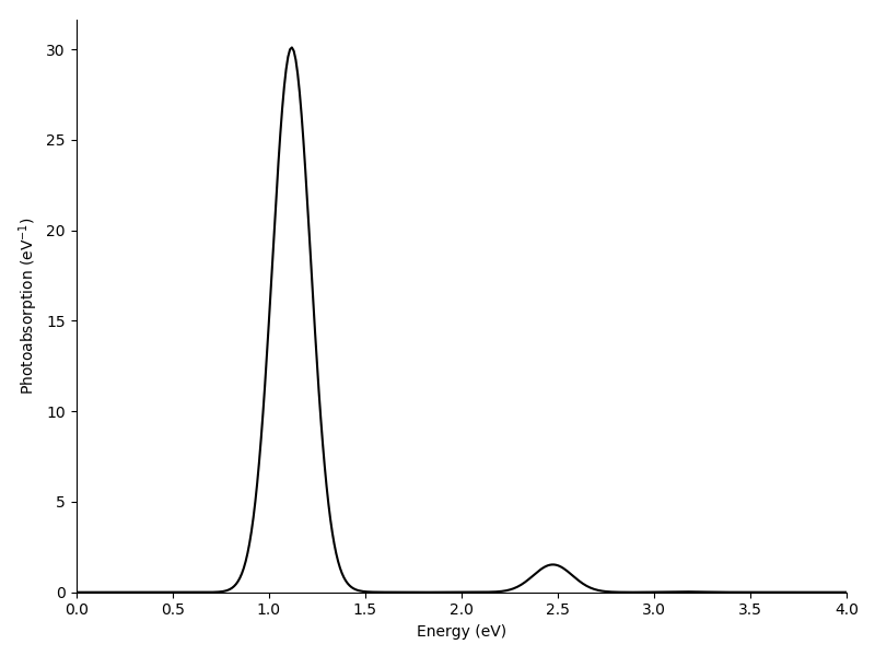
The two main resonances are analyzed in the following.
Frequency-space density matrix
We generate the density matrix for the frequencies of interest:
from gpaw.lcaotddft import LCAOTDDFT
from gpaw.lcaotddft.densitymatrix import DensityMatrix
from gpaw.lcaotddft.frequencydensitymatrix import FrequencyDensityMatrix
from gpaw.tddft.folding import frequencies

# Read the ground-state file
td_calc = LCAOTDDFT('gs.gpw')

# Attach analysis tools
dmat = DensityMatrix(td_calc)
freqs = frequencies([1.12, 2.48], 'Gauss', 0.1)
fdm = FrequencyDensityMatrix(td_calc, dmat, frequencies=freqs)

# Replay the propagation
td_calc.replay(name='wf.ulm', update='none')

# Store the density matrix
fdm.write('fdm.ulm')
Transform the density matrix to Kohn–Sham electron-hole basis
First, we construct the Kohn–Sham electron-hole basis. For that we need to calculate unoccupied Kohn–Sham states, which is conveniently done by restarting from the earlier ground-state file:
from gpaw import GPAW
from gpaw.lcaotddft.ksdecomposition import KohnShamDecomposition

# Calculate ground state with full unoccupied space
calc = GPAW('gs.gpw', txt=None).fixed_density(nbands='nao', txt='unocc.out')
calc.write('unocc.gpw', mode='all')

# Construct KS electron-hole basis
ksd = KohnShamDecomposition(calc)
ksd.initialize(calc)
ksd.write('ksd.ulm')
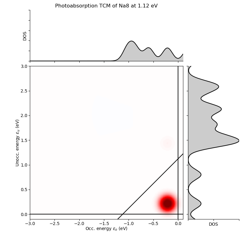
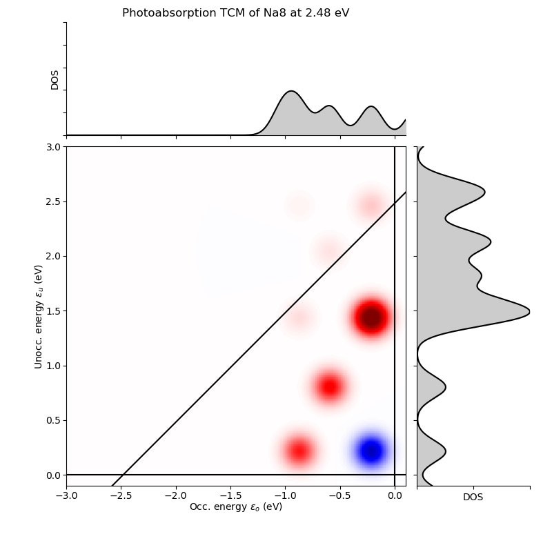
Next, we can use the created objects to transform the LCAO density matrix to the Kohn–Sham electron-hole basis and visualize the photoabsorption decomposition as a transition contribution map (TCM):
# web-page: tcm_1.12.png, tcm_2.48.png, table_1.12.txt, table_2.48.txt
import numpy as np
from matplotlib import pyplot as plt

from gpaw import GPAW
from gpaw.tddft.units import au_to_eV
from gpaw.lcaotddft.ksdecomposition import KohnShamDecomposition
from gpaw.lcaotddft.densitymatrix import DensityMatrix
from gpaw.lcaotddft.frequencydensitymatrix import FrequencyDensityMatrix
from gpaw.lcaotddft.tcm import TCMPlotter

# Load the objects
calc = GPAW('unocc.gpw', txt=None)
ksd = KohnShamDecomposition(calc, 'ksd.ulm')
dmat = DensityMatrix(calc)
fdm = FrequencyDensityMatrix(calc, dmat, 'fdm.ulm')

plt.figure(figsize=(8, 8))


def do(w):
    # Select the frequency and the density matrix
    rho_uMM = fdm.FReDrho_wuMM[w]
    freq = fdm.freq_w[w]
    frequency = freq.freq * au_to_eV
    print(f'Frequency: {frequency:.2f} eV')
    print(f'Folding: {freq.folding}')

    # Transform the LCAO density matrix to KS basis
    rho_up = ksd.transform(rho_uMM)

    # Photoabsorption decomposition
    dmrho_vp = ksd.get_dipole_moment_contributions(rho_up)
    weight_p = 2 * freq.freq / np.pi * dmrho_vp[0].imag / au_to_eV * 1e5
    print(f'Total absorption: {np.sum(weight_p):.2f} eV^-1')

    # Print contributions as a table
    table = ksd.get_contributions_table(weight_p, minweight=0.1)
    print(table)
    with open(f'table_{frequency:.2f}.txt', 'w') as f:
        f.write(f'Frequency: {frequency:.2f} eV\n')
        f.write(f'Folding: {freq.folding}\n')
        f.write(f'Total absorption: {np.sum(weight_p):.2f} eV^-1\n')
        f.write(table)

    # Plot the decomposition as a TCM
    de = 0.01
    energy_o = np.arange(-3, 0.1 + 1e-6, de)
    energy_u = np.arange(-0.1, 3 + 1e-6, de)
    plt.clf()
    plotter = TCMPlotter(ksd, energy_o, energy_u, sigma=0.1)
    plotter.plot_TCM(weight_p)
    plotter.plot_DOS(fill={'color': '0.8'}, line={'color': 'k'})
    plotter.plot_TCM_diagonal(freq.freq * au_to_eV, color='k')
    plotter.set_title(f'Photoabsorption TCM of Na8 at {frequency:.2f} eV')

    # Check that TCM integrates to correct absorption
    tcm_ou = ksd.get_TCM(weight_p, ksd.get_eig_n()[0],
                         energy_o, energy_u, sigma=0.1)
    print(f'TCM absorption: {np.sum(tcm_ou) * de ** 2:.2f} eV^-1')

    # Save the plot
    plt.savefig(f'tcm_{frequency:.2f}.png')


do(0)
do(1)
Note that the sum over the decomposition (the printed total absorption) equals to the value of the photoabsorption spectrum at the particular frequency in question.
We obtain the following transition contributions for the resonances (presented both as tables and TCMs):
Frequency: 1.12 eV
Folding: Gauss(0.10000 eV)
Total absorption: 30.11 eV^-1
#      p    i(      eV)       a(      eV)    Ediff (eV)         weight        %
       0    3(  -0.214) ->    4(   0.214):       0.4279        29.2938     97.3
       6    3(  -0.214) ->    6(   1.434):       1.6479         0.5588      1.9
      36    3(  -0.214) ->   16(   2.456):       2.6696         0.1294      0.4
       5    2(  -0.593) ->    5(   0.801):       1.3943         0.1199      0.4
                                     rest:                     +0.0074      0.0
                                    total:                    +30.1092    100.0
Frequency: 2.48 eV
Folding: Gauss(0.10000 eV)
Total absorption: 1.53 eV^-1
#      p    i(      eV)       a(      eV)    Ediff (eV)         weight        %
       6    3(  -0.214) ->    6(   1.434):       1.6479         1.0450     68.4
       0    3(  -0.214) ->    4(   0.214):       0.4279        -0.5812    -38.0
       5    2(  -0.593) ->    5(   0.801):       1.3943         0.4450     29.1
       3    1(  -0.871) ->    4(   0.214):       1.0853         0.3866     25.3
                                     rest:                     +0.2332     15.3
                                    total:                     +1.5286    100.0
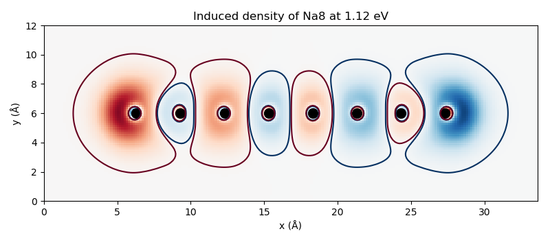
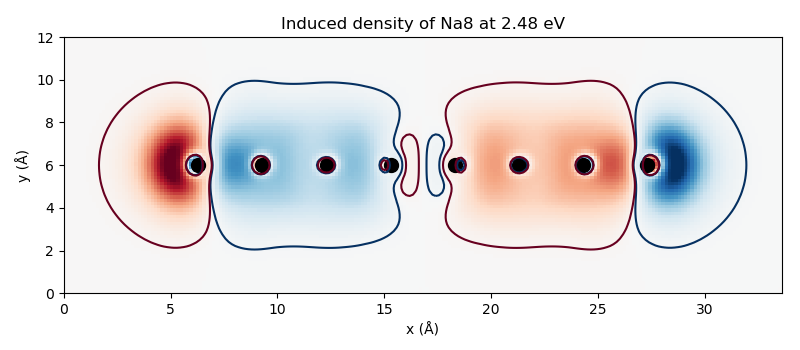
Induced density
The density matrix gives access to any other quantities. For instance, the induced density can be conveniently obtained from the density matrix:
import numpy as np

from ase.io import write
from gpaw import GPAW
from gpaw.tddft.units import au_to_eV
from gpaw.lcaotddft.densitymatrix import DensityMatrix
from gpaw.lcaotddft.frequencydensitymatrix import FrequencyDensityMatrix

# Load the objects
calc = GPAW('unocc.gpw', txt=None)
calc.initialize_positions()  # Initialize in order to calculate density
dmat = DensityMatrix(calc)
fdm = FrequencyDensityMatrix(calc, dmat, 'fdm.ulm')


def do(w):
    # Select the frequency and the density matrix
    rho_MM = fdm.FReDrho_wuMM[w][0]
    freq = fdm.freq_w[w]
    frequency = freq.freq * au_to_eV
    print(f'Frequency: {frequency:.2f} eV')
    print(f'Folding: {freq.folding}')

    # Induced density
    rho_g = dmat.get_density([rho_MM.imag])

    # Save as a cube file
    write(f'ind_{frequency:.2f}.cube', calc.atoms, data=rho_g)

    # Calculate dipole moment for reference
    dm_v = dmat.density.finegd.calculate_dipole_moment(rho_g, center=True)
    absorption = 2 * freq.freq / np.pi * dm_v[0] / au_to_eV * 1e5
    print(f'Total absorption: {absorption:.2f} eV^-1')


do(0)
do(1)
The resulting cube files can be visualized, for example, with
this script producing
the figures:
Advanced tutorials
Plasmon resonance of silver cluster
In this tutorial, we demonstrate the use of
efficient parallelization settings and
calculate the photoabsorption spectrum of
an icosahedral Ag55 cluster.
We use GLLB-SC potential to significantly improve the description of d states,
p-valence basis sets to improve the description of unoccupied states, and
11-electron Ag setup to reduce computational cost.
When calculating other systems, remember to check the convergence with respect to the used basis sets. Recall hints here.
The workflow is the same as in the previous examples. First, we calculate ground state (takes around 20 minutes with 36 cores):
from ase.io import read
from gpaw import GPAW, FermiDirac, Mixer, PoissonSolver
from gpaw.poisson_moment import MomentCorrectionPoissonSolver

# Read the structure from the xyz file
atoms = read('Ag55.xyz')
atoms.center(vacuum=6.0)

# Increase the accuracy of density for ground state
convergence = {'density': 1e-12}

# Use occupation smearing, weak mixer and GLLB weight smearing
# to facilitate convergence
occupations = FermiDirac(25e-3)
mixer = Mixer(0.02, 5, 1.0)
xc = 'GLLBSC:width=0.002'

# Parallelzation settings
parallel = {'sl_auto': True, 'domain': 2, 'augment_grids': True}

# Apply multipole corrections for monopole and dipoles
poissonsolver = MomentCorrectionPoissonSolver(poissonsolver=PoissonSolver(),
                                              moment_corrections=1 + 3)

# Ground-state calculation
calc = GPAW(mode='lcao', xc=xc, h=0.3, nbands=360,
            setups={'Ag': '11'},
            basis={'Ag': 'pvalence.dz', 'default': 'dzp'},
            convergence=convergence, poissonsolver=poissonsolver,
            occupations=occupations, mixer=mixer, parallel=parallel,
            maxiter=1000,
            txt='gs.out',
            symmetry={'point_group': False})
atoms.calc = calc
atoms.get_potential_energy()
calc.write('gs.gpw', mode='all')
Then, we carry the time propagation for 30 femtoseconds in steps of 10 attoseconds (takes around 3.5 hours with 36 cores):
from gpaw.lcaotddft import LCAOTDDFT
from gpaw.lcaotddft.dipolemomentwriter import DipoleMomentWriter

# Parallelzation settings
parallel = {'sl_auto': True, 'domain': 2, 'augment_grids': True}

# Time propagation
td_calc = LCAOTDDFT('gs.gpw', parallel=parallel, txt='td.out')
DipoleMomentWriter(td_calc, 'dm.dat')
td_calc.absorption_kick([1e-5, 0.0, 0.0])
td_calc.propagate(10, 3000)
Finally, we calculate the spectrum (takes a few seconds):
from gpaw.tddft.spectrum import photoabsorption_spectrum

# Calculate spectrum
photoabsorption_spectrum('dm.dat', 'spec.dat', width=0.1, delta_e=0.01)
The resulting spectrum shows an emerging plasmon resonance at around 4 eV:
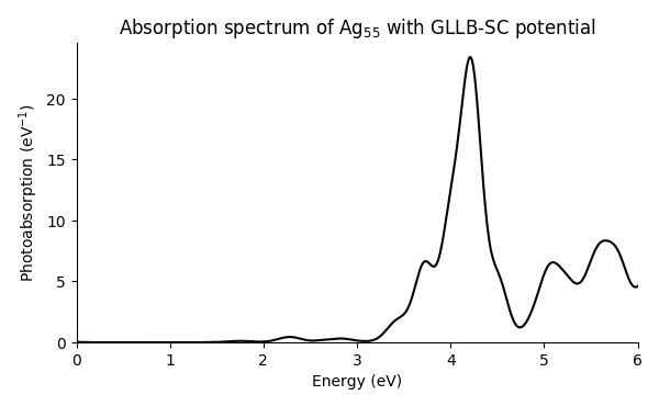
For further insight on plasmon resonance in metal nanoparticles, see [1] and [3].
User-generated basis sets
The p-valence basis sets distributed with GPAW and used in the above tutorial have been generated from atomic PBE orbitals. Similar basis sets can be generated based on atomic GLLB-SC orbitals:
from gpaw.atom.generator import Generator
from gpaw.atom.basis import BasisMaker
from gpaw.atom.configurations import parameters, parameters_extra

atom = 'Ag'
xc = 'GLLBSC'
name = 'my'
if atom in parameters_extra:
    args = parameters_extra[atom]  # Choose the smaller setup
else:
    args = parameters[atom]  # Choose the larger setup
args.update(dict(name=name, exx=True))

# Generate setup
generator = Generator(atom, xc, scalarrel=True)
generator.run(write_xml=True, **args)

# Generate basis
bm = BasisMaker(atom, name=f'{name}.{xc}', xc=xc, run=False)
bm.generator.run(write_xml=False, **args)
basis = bm.generate(zetacount=2, polarizationcount=0,
                    jvalues=[0, 1, 2])  # include d, s and p
basis.write_xml()
The Ag55 cluster can be calculated as in the above tutorial, once the input scripts have been modified to use the generated setup and basis set. Changes to the ground-state script:
--- /scratch/jensj/gpaw-docs/gpaw/doc/tutorialsexercises/opticalresponse/tddft/lcaotddft_Ag55/gs.py
+++ /scratch/jensj/gpaw-docs/gpaw/doc/tutorialsexercises/opticalresponse/tddft/lcaotddft_Ag55/mybasis/gs.py
@@ -1,6 +1,10 @@
 from ase.io import read
 from gpaw import GPAW, FermiDirac, Mixer, PoissonSolver
+from gpaw import setup_paths
 from gpaw.poisson_moment import MomentCorrectionPoissonSolver
+
+# Insert the path to the created basis set
+setup_paths.insert(0, '.')

 # Read the structure from the xyz file
 atoms = read('Ag55.xyz')
@@ -24,8 +28,8 @@

 # Ground-state calculation
 calc = GPAW(mode='lcao', xc=xc, h=0.3, nbands=360,
-            setups={'Ag': '11'},
-            basis={'Ag': 'pvalence.dz', 'default': 'dzp'},
+            setups={'Ag': 'my'},
+            basis={'Ag': 'GLLBSC.dz', 'default': 'dzp'},
             convergence=convergence, poissonsolver=poissonsolver,
             occupations=occupations, mixer=mixer, parallel=parallel,
             maxiter=1000,
Changes to the time-propagation script:
--- /scratch/jensj/gpaw-docs/gpaw/doc/tutorialsexercises/opticalresponse/tddft/lcaotddft_Ag55/td.py
+++ /scratch/jensj/gpaw-docs/gpaw/doc/tutorialsexercises/opticalresponse/tddft/lcaotddft_Ag55/mybasis/td.py
@@ -1,5 +1,9 @@
 from gpaw.lcaotddft import LCAOTDDFT
 from gpaw.lcaotddft.dipolemomentwriter import DipoleMomentWriter
+from gpaw import setup_paths
+
+# Insert the path to the created basis set
+setup_paths.insert(0, '.')

 # Parallelzation settings
 parallel = {'sl_auto': True, 'domain': 2, 'augment_grids': True}
The calculation with this generated “my” p-valence basis set results only in small differences in the spectrum in comparison to the distributed p-valence basis sets:
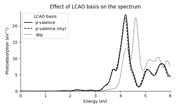
The spectrum with the default dzp basis sets is also shown for reference, resulting in unconverged spectrum due to the lack of diffuse functions. This demonstrates the importance of checking convergence with respect to the used basis sets. Recall hints here and see [1] and [2] for further discussion on the basis sets.
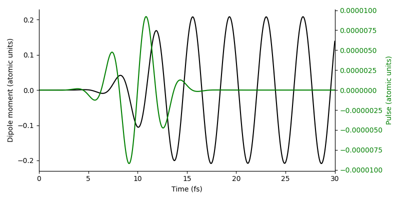
Time-dependent potential
Instead of using the dipolar delta kick as a time-domain perturbation, it is possible to define any time-dependent potential.
Considering the sodium atom chain as an example, we can tune a dipolar Gaussian pulse to its resonance at 1.12 eV and propagate the system:
import numpy as np
from ase.units import Hartree, Bohr
from gpaw.external import ConstantElectricField
from gpaw.lcaotddft import LCAOTDDFT
from gpaw.lcaotddft.laser import GaussianPulse
from gpaw.lcaotddft.dipolemomentwriter import DipoleMomentWriter

# Temporal shape of the time-dependent potential
pulse = GaussianPulse(1e-5, 10e3, 1.12, 0.3, 'sin')
# Spatial shape of the time-dependent potential
ext = ConstantElectricField(Hartree / Bohr, [1., 0., 0.])
# Full time-dependent potential
td_potential = {'ext': ext, 'laser': pulse}

# Write the temporal shape to a file
pulse.write('pulse.dat', np.arange(0, 30e3, 10.0))

# Set up the time-propagation calculation
td_calc = LCAOTDDFT('gs.gpw', td_potential=td_potential,
                    txt='tdpulse.out')

# Attach the data recording and analysis tools
DipoleMomentWriter(td_calc, 'dmpulse.dat')

# Propagate
td_calc.propagate(20, 1500)

# Save the state for restarting later
td_calc.write('tdpulse.gpw', mode='all')
The resulting dipole-moment response shows the resonant excitation of the system:
References
Code documentation
Observers
- class gpaw.lcaotddft.dipolemomentwriter.DipoleMomentWriter(paw, filename, *, center=False, density='comp', force_new_file=False, interval=1)[source]
Observer for writing time-dependent dipole moment data.
The data is written in atomic units.
The observer attaches to the TDDFT calculator during creation.
- Parameters:
paw – TDDFT calculator
filename (str) – File for writing dipole moment data
center (bool) – If true, dipole moment is evaluated with the center of cell as the origin
density (str) – Density type used for evaluating dipole moment. Use the default value for production calculations; others are for testing purposes. Possible values:
'comp':rhot_g,'pseudo':nt_sg,'pseudocoarse':nt_sG.force_new_file (bool) – If true, new dipole moment file is created (erasing any existing one) even when restarting time propagation.
interval (int) – Update interval. Value of 1 corresponds to evaluating and writing data after every propagation step.