The Quantum Electrostatic Heterostructure (QEH) model

Brief overview

In this tuturial we show how to calculate the linear response of a general van der Waals Heterostructure (vdWH) by means of the quantum electrostatic heterostructure (QEH) model. This method allows to overcome the computational limitation of the standard ab-initio approaches by combining quantum accuracy at the monolayer level and macroscopic electrostatic coupling between the layers. More specifically, the first step consists in calculating the response function of each of the layers composing the vdWHs in the isolated condition and encoding it into a so called dielectric building block. Then, in the next step the dielectric building blocks are coupled together through a macroscopic Dyson equation. The validity of such an approach strongly relies on the absence of hybridization among the layers, condition which is usually satisfied by vdWHs.

A thourough description of the QEH model can be found in [1] and [2]:

[1]

K. Andersen, S. Latini and K.S. Thygesen Dielectric genome of van der Waals heterostructures Nano Letters 15 (7), 4616-4621 (2015)

[2]

M. N. Gjerding, L. S. R. Cavalcante, Andrey Chaves, and K. S. Thygesen Efficient Ab Initio Modeling of Dielectric Screening in 2D van der Waals Materials: Including Phonons, Substrates, and Doping J. Phys. Chem. C 2020, 124, 21, 11609–11616

See also

• Documentation for the qeh Python package.

• qeh on PyPI.

• Examples from the CMR database.

Constructing a dielectric building block

First, we need a ground state calculation for each of the layers in the vdWH. We will consider a MoS2/WSe2 bilayer. In the following script we show how to get the ground state gpw-file for the MoS2 layer:

from ase.build import mx2
from gpaw import GPAW, PW, FermiDirac


structure = mx2(formula='MoS2', kind='2H', a=3.184, thickness=3.127,
                size=(1, 1, 1), vacuum=5)

ecut = 600

calc = GPAW(mode=PW(ecut),
            xc='LDA',
            kpts={'size': (30, 30, 1), 'gamma': True},
            occupations=FermiDirac(0.01),
            parallel={'domain': 1},
            txt='MoS2_gs_out.txt')

structure.calc = calc
structure.get_potential_energy()

calc.diagonalize_full_hamiltonian(nbands=500, expert=True)
calc.write('MoS2_gs_fulldiag.gpw', 'all')

The gpw-file for WSe2 can be obtained in a similar way. The gpw-files stores all the necessary eigenvalues and eigenfunctions for the response calculation.

Next the building blocks are created by using the BuildingBlock class. Essentially, a Dyson equation for the isolated layer is solved to obtain the full response function \(\chi(q,\omega)\). Starting from \(\chi(q,\omega)\) the monopole and dipole component of the response function and of the induced densities are condensed into the dielectric building block. Here is how to get the MoS2 and building block:

from pathlib import Path
from gpaw.mpi import world
from gpaw.response.df import DielectricFunction
from gpaw.response.qeh import BuildingBlock

df = DielectricFunction(calc='MoS2_gs_fulldiag.gpw',
                        eta=0.001,
                        frequencies={'type': 'nonlinear',
                                     'domega0': 0.05,
                                     'omega2': 10.0},
                        nblocks=8,
                        ecut=150,
                        truncation='2D')

buildingblock = BuildingBlock('MoS2', df, qmax=3.0)

buildingblock.calculate_building_block()

if world.rank == 0:
    Path('MoS2_gs_fulldiag.gpw').unlink()

The same goes for the WSe2 building block. Once the building blocks have been created, they need to be interpolated to the same kpoint and frequency grid. This is done as follows:

from qeh import interpolate_building_blocks
interpolate_building_blocks(BBfiles=['WSe2'], BBmotherfile='MoS2')

Specifically, this interpolates the WSe2 building block to the MoS2 grid.

Finally the building blocks are ready to be combined electrostatically.

Interlayer excitons in MoS2/WSe2

As shown in [3] the MoS2_WSe2 can host excitonic excitations where the electron and the hole are spatially separated, with the electron sitting in the MoS2 layer and the hole in the WSe2 one.

Because of the finite separation distance we expect that the electron-hole screened interaction between the two particles will not diverge when the in-plane separation goes to 0. To illustrate this we show how to calculate the screened electron-hole interaction using the QEH model and the building blocks created above:

# web-page: W_r.svg
import numpy as np
import matplotlib.pyplot as plt
from qeh import Heterostructure


thick_MoS2 = 6.2926
thick_WSe2 = 6.718

d_MoS2_WSe2 = (thick_MoS2 + thick_WSe2) / 2
inter_mass = 0.244

HS = Heterostructure(structure=['MoS2_int', 'WSe2_int'],
                     d=[d_MoS2_WSe2],
                     qmax=None,
                     wmax=0,
                     d0=thick_WSe2)

hl_array = np.array([0., 0., 1., 0.])
el_array = np.array([1., 0., 0., 0.])


# Getting the interlayer exciton screened interaction on a real grid
r, W_r = HS.get_exciton_screened_potential_r(
    r_array=np.linspace(1e-1, 30, 1000),
    e_distr=el_array,
    h_distr=hl_array)

plt.plot(r, W_r, '-g')
plt.title(r'Screened Interaction Energy')
plt.xlabel(r'${\bf r}$ (Ang)', fontsize=20)
plt.ylabel(r'$W({\bf r})$ (Ha)', fontsize=20)
plt.savefig('W_r.svg')
plt.show()

Here is the generated plot:

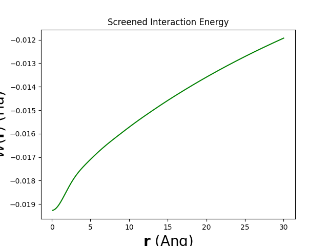
As expected the interaction does not diverge.

If one is also interested in the interlayer exciton binding energy, it can be readily calculated by appending the following lines in the script above:

ee, ev = HS.get_exciton_binding_energies(eff_mass=inter_mass,
                                         e_distr=el_array,
                                         h_distr=hl_array)

print('The interlayer exciton binding energy is:', -ee[0])

We find an interlayer exciton binding energy of \(\sim 0.3\) eV.

[3]

S. Latini, K.T. Winther, T. Olsen and K.S. Thygesen Interlayer Excitons and Band Alignment in MoS2/hBN/WSe2 van der Waals Heterostructures Nano Letters Just accepted (2017)