Linear response TDDFT 2 - indexed version
Ground state
The linear response TDDFT calculation needs a converged ground state calculation with a set of unoccupied states.
We demonstrate the code usage for
(R)-methyloxirane molecule.
First, we calculate the ground state:
from ase.io import read
from gpaw import GPAW

atoms = read('r-methyloxirane.xyz')
atoms.center(vacuum=8)

calc = GPAW(mode='fd',
            h=0.2,
            nbands=14,
            xc='LDA',
            poissonsolver={'name': 'MomentCorrectionPoissonSolver',
                           'poissonsolver': 'fast',
                           'moment_corrections': 1 + 3 + 5},
            convergence={'bands': 'occupied'},
            txt='gs.out')
atoms.calc = calc
atoms.get_potential_energy()
calc.write('gs.gpw', mode='all')
Text output: gs.out.
Then, we converge unoccupied states:
from gpaw import GPAW

calc = GPAW('gs.gpw')
calc = calc.fixed_density(nbands=42,
                          convergence={'bands': 40},
                          maxiter=1000,
                          txt='unocc.out')
calc.write('unocc.gpw', mode='all')
Text output: unocc.out.
Let’s have a look on the states in the output file:
 Band  Eigenvalues  Occupancy
    0    -27.01684    2.00000
    1    -18.44358    2.00000
    2    -16.21613    2.00000
    3    -14.70939    2.00000
    4    -12.66138    2.00000
    5    -11.68439    2.00000
    6    -10.60330    2.00000
    7     -9.93510    2.00000
    8     -9.26324    2.00000
    9     -8.94170    2.00000
   10     -7.44985    2.00000
   11     -6.29526    2.00000
   12     -0.43775    0.00000
   13      0.01845    0.00000
   14      0.03453    0.00000
   15      0.14067    0.00000
   16      0.63631    0.00000
   17      0.67821    0.00000
   18      0.71377    0.00000
   19      0.82988    0.00000
   20      0.86534    0.00000
   21      0.90683    0.00000
   22      1.00434    0.00000
   23      1.02512    0.00000
   24      1.06549    0.00000
   25      1.19626    0.00000
   26      1.27747    0.00000
   27      1.34996    0.00000
   28      1.37359    0.00000
   29      1.41483    0.00000
   30      1.43999    0.00000
   31      1.47051    0.00000
   32      1.53497    0.00000
   33      1.58404    0.00000
   34      1.63794    0.00000
   35      1.66528    0.00000
   36      1.71123    0.00000
   37      1.79165    0.00000
   38      1.83837    0.00000
   39      1.86016    0.00000
   40      1.89781    0.00000
   41      1.99247    0.00000
We see that the Kohn-Sham eigenvalue difference between HOMO and the highest converged unoccupied state is about 8.2 eV. Thus, all Kohn-Sham single-particle transitions up to this energy difference can be calculated from these unoccupied states. If more is needed, then more unoccupied states would need to be converged.
Note
Converging unoccupied states in some systems may require tuning the eigensolver. See the possible options in the manual.
Calculating response matrix and spectrum
The next step is to calculate the response matrix with
LrTDDFT2.
A very important convergence parameter is the number of Kohn-Sham
single-particle transitions used to calculate the response matrix.
This can be set through state indices
(see the parameters of LrTDDFT2),
or as demonstrated here,
through an energy cutoff parameter max_energy_diff.
This parameter defines the maximum energy difference of
the Kohn-Sham transitions included in the calculation.
Note! If the used gpw file does not contain enough unoccupied states so
that all single-particle transitions defined by max_energy_diff
can be included, then the calculation does not usually make sense.
Thus, check carefully the states in the unoccupied states calculation
(see the example above).
Note also! The max_energy_diff parameter does not mean that
the TDDFT excitations would be converged up to this energy.
Typically, the max_energy_diff needs to be much larger than the smallest
excitation energy of interest to obtain well converged results.
Checking the convergence with respect to the number of states
included in the calculation is crucial.
In this script, we set max_energy_diff to 7 eV.
We also show how to parallelize calculation
over Kohn-Sham electron-hole (eh) pairs with
LrCommunicators
(8 tasks are used for each GPAW calculator):
from gpaw.mpi import world
from gpaw import GPAW
from gpaw.lrtddft2 import LrTDDFT2
from gpaw.lrtddft2.lr_communicators import LrCommunicators

# Maximum energy difference for Kohn-Sham transitions
# included in the calculation
max_energy_diff = 7.0  # eV

# Set parallelization
dd_size = 2 * 2 * 2
eh_size = world.size // dd_size
assert eh_size * dd_size == world.size
lr_comms = LrCommunicators(world, dd_size, eh_size)

calc = GPAW('unocc.gpw',
            communicator=lr_comms.dd_comm)
lr = LrTDDFT2('lr2', calc,
              fxc='LDA',
              max_energy_diff=max_energy_diff,
              recalculate=None,  # Change this to force recalculation
              lr_communicators=lr_comms,
              txt='lr2_with_%05.2feV.out' % max_energy_diff)

# This is the expensive part triggering the calculation!
lr.calculate()

# Get and write spectrum
spec = lr.get_spectrum('spectrum_with_%05.2feV.dat'
                       % max_energy_diff,
                       min_energy=0,
                       max_energy=10,
                       energy_step=0.01,
                       width=0.1)

# Get and write transitions
trans = lr.get_transitions('transitions_with_%05.2feV.dat'
                           % max_energy_diff,
                           min_energy=0.0,
                           max_energy=10.0)
Text output (lr2_with_07.00eV.out)
shows the number of Kohn-Sham transitions within the set 7 eV limit:
Number of electron-hole pairs: 6
Maximum energy difference:      6.973
Calculating spectrum    (2024-07-23 11:47:31.234765).
Spectrum calculated     (2024-07-23 11:47:31.256380).
Calculating transitions (2024-07-23 11:47:31.277754).
Transitions calculated  (2024-07-23 11:47:31.294397).
The TDDFT excitations are
(transitions_with_07.00eV.dat):
#       energy       osc str       rot str        osc str x     osc str y     osc str z    units: eVcgs
    5.90014859    0.01415298  -22.29693665       0.00454107    0.00651019    0.03140768
    6.31736848    0.03467841   14.60027850       0.02842660    0.00920665    0.06640197
    6.36238701    0.01720349    3.39489696       0.02010759    0.01895798    0.01254491
    6.48395718    0.00716565    2.79810861       0.00023825    0.00011389    0.02114480
    6.94316199    0.00763759    3.06134039       0.00220299    0.01634170    0.00436809
    7.00422991    0.00557088   -1.47973671       0.01088486    0.00165336    0.00417441
Restarting and recalculating
The calculation can be restarted with the same scipt. As an example, here we increase the energy cutoff to 8 eV. The matrix elements calculated earlier up to 7 eV are reused, and only the missing matrix elements are calculated:
from gpaw.mpi import world
from gpaw import GPAW
from gpaw.lrtddft2 import LrTDDFT2
from gpaw.lrtddft2.lr_communicators import LrCommunicators

# Maximum energy difference for Kohn-Sham transitions
# included in the calculation
max_energy_diff = 8.0  # eV

# Set parallelization
dd_size = 2 * 2 * 2
eh_size = world.size // dd_size
assert eh_size * dd_size == world.size
lr_comms = LrCommunicators(world, dd_size, eh_size)

calc = GPAW('unocc.gpw',
            communicator=lr_comms.dd_comm)
lr = LrTDDFT2('lr2', calc,
              fxc='LDA',
              max_energy_diff=max_energy_diff,
              recalculate=None,  # Change this to force recalculation
              lr_communicators=lr_comms,
              txt='lr2_with_%05.2feV.out' % max_energy_diff)

# This is the expensive part triggering the calculation!
lr.calculate()

# Get and write spectrum
spec = lr.get_spectrum('spectrum_with_%05.2feV.dat'
                       % max_energy_diff,
                       min_energy=0,
                       max_energy=10,
                       energy_step=0.01,
                       width=0.1)

# Get and write transitions
trans = lr.get_transitions('transitions_with_%05.2feV.dat'
                           % max_energy_diff,
                           min_energy=0.0,
                           max_energy=10.0)
Text output (lr2_with_08.00eV.out)
shows the number of Kohn-Sham transitions within the set limit:
Number of electron-hole pairs: 28
Maximum energy difference:      7.961
Calculating spectrum    (2024-07-23 11:49:14.256317).
Spectrum calculated     (2024-07-23 11:49:14.298392).
Calculating transitions (2024-07-23 11:49:14.341338).
Transitions calculated  (2024-07-23 11:49:14.372377).
The TDDFT excitations are
(transitions_with_08.00eV.dat):
#       energy       osc str       rot str        osc str x     osc str y     osc str z    units: eVcgs
    5.89434225    0.01286016  -22.38635506       0.00467060    0.00433082    0.02957905
    6.31647544    0.03382317   14.26689240       0.02727170    0.00916365    0.06503416
    6.35484909    0.01351514    1.51511653       0.01876752    0.01279369    0.00898422
    6.47796623    0.00636743    2.73730580       0.00037130    0.00014909    0.01858190
    6.93880615    0.00685675    1.21787987       0.00109041    0.01398186    0.00549798
    6.99529312    0.00416800   -1.06399455       0.00787600    0.00276062    0.00186738
    7.00273395    0.00197321   -1.12516854       0.00020712    0.00560001    0.00011251
    7.05405681    0.00784394    7.18697089       0.01310312    0.00970403    0.00072468
    7.13526003    0.00154719   -0.79668563       0.00084143    0.00023426    0.00356589
    7.16399561    0.00312080   -1.29659902       0.00469785    0.00406846    0.00059610
    7.22806831    0.00171861   -0.15082791       0.00000630    0.00000010    0.00514944
    7.32175725    0.01331729    9.18718220       0.00011708    0.00621724    0.03361755
    7.35667273    0.00338142   -3.72182325       0.00596230    0.00002769    0.00415426
    7.38311944    0.00988269    9.30243311       0.02726894    0.00020590    0.00217322
    7.48875052    0.00646825   -1.75481612       0.00004130    0.01487458    0.00448887
    7.49725391    0.00010539   -0.01049470       0.00013052    0.00006307    0.00012257
    7.52261324    0.01096163   -7.77486521       0.00756206    0.00082819    0.02449464
    7.61452934    0.00005488   -0.88697091       0.00006544    0.00000277    0.00009643
    7.64617018    0.00446563    0.94474977       0.00562240    0.00001166    0.00776282
    7.68148265    0.00069125   -0.59267925       0.00137820    0.00006153    0.00063400
    7.72419854    0.01576408   -4.16098196       0.01281219    0.03447988    0.00000016
    7.75473167    0.01454875   -3.37320560       0.01581073    0.02741790    0.00041763
    7.77425369    0.01075815   11.02353811       0.00394681    0.02830612    0.00002151
    7.78502206    0.01614515   -6.84563210       0.03035132    0.01033524    0.00774889
    7.85456975    0.01031334   -1.88762742       0.00002036    0.02874120    0.00217847
    7.90796673    0.01391711    3.10345808       0.00002103    0.04115467    0.00057563
    7.95224825    0.01915341    7.02216480       0.00001059    0.05570213    0.00174753
    8.01054300    0.00659157    6.37302272       0.01063884    0.00314393    0.00599195
It’s important to note that also the first excitations change in comparison to the earlier calculation with the 7 eV cutoff energy. As stated earlier, the results must be converged with respect to the cutoff energy, and typically the cutoff energy needs to be much larger than the smallest excitation energy of interest.
Here we plot the photoabsorption and rotatory strength spectra from
the data files (
spectrum_with_07.00eV.dat and
spectrum_with_08.00eV.dat):
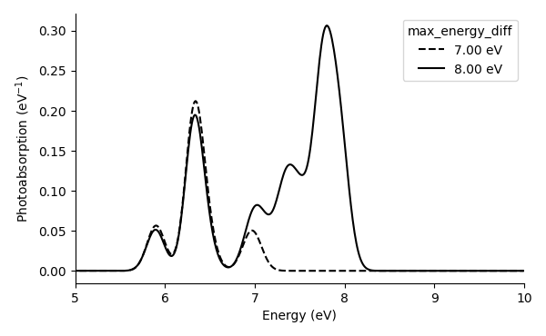
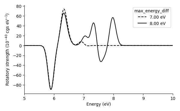
We note that the cutoff energy (and the number of unoccupied bands) should be increased more to converge the spectra properly.
Analyzing spectrum
Once the response matrix has been calculated, the same input script can be used for calculating the spectrum and analyzing the transitions. But, as all the expensive calculation is done already, it’s sufficient to run the script in serial. Here is an example script for analysis without parallelization settings:
from ase.parallel import paropen
from gpaw import GPAW
from gpaw.lrtddft2 import LrTDDFT2

# Maximum energy difference for Kohn-Sham transitions
# included in the calculation
max_energy_diff = 8.0  # eV

calc = GPAW('unocc.gpw')
lr = LrTDDFT2('lr2', calc,
              fxc='LDA',
              max_energy_diff=max_energy_diff,
              txt='-')

# Get and write spectrum
spec = lr.get_spectrum('spectrum_with_%05.2feV.dat'
                       % max_energy_diff,
                       min_energy=0,
                       max_energy=10,
                       energy_step=0.01,
                       width=0.1)

# Get and write transitions
trans = lr.get_transitions('transitions_with_%05.2feV.dat'
                           % max_energy_diff,
                           min_energy=0.0,
                           max_energy=10.0)

# Get and write transition contributions
index = 0
f2 = lr.get_transition_contributions(index_of_transition=index)
with paropen('tc_%03d_with_%05.2feV.txt'
             % (index, max_energy_diff), 'w') as f:
    f.write('Transition %d at %.2f eV\n' % (index, trans[0][index]))
    f.write(' %5s => %5s  contribution\n' % ('occ', 'unocc'))
    for (ip, val) in enumerate(f2):
        if (val > 1e-3):
            f.write(' %5d => %5d  %8.4f%%\n' %
                    (lr.ks_singles.kss_list[ip].occ_ind,
                     lr.ks_singles.kss_list[ip].unocc_ind,
                     val / 2. * 100))
The script produces the same spectra and transitions as above.
In addition, it demonstrates how to analyze transition contributions.
An example for the first TDDFT excitation
(tc_000_with_08.00eV.txt):
Transition 0 at 5.89 eV
   occ => unocc  contribution
    11 =>    12   99.0869%
    11 =>    13    0.0875%
    11 =>    14    0.3664%
    11 =>    15    0.1311%
    11 =>    19    0.0534%
Note that while this excitation is at about 5.9 eV, it has non-negligible
contributions from Kohn-Sham single-particle transitions above this energy.
This is generally the case, and it is basically the reason why
the max_energy_diff parameter has to be typically much higher
than the highest excitation energies of interest.
Quick reference
- class gpaw.lrtddft2.LrTDDFT2(basefilename, gs_calc, fxc=None, min_occ=None, max_occ=None, min_unocc=None, max_unocc=None, max_energy_diff=None, recalculate=None, lr_communicators=None, txt='-')[source]
Linear response TDDFT (Casida) class with indexed K-matrix storage.
Initialize linear response TDDFT without calculating anything.
Note
Does NOT support spin polarized calculations yet.
Tip
If K_matrix file is too large and you keep running out of memory when trying to calculate spectrum or response wavefunction, you can try
split -l 100000 xxx.K_matrix.ddddddofDDDDDD xxx.K_matrix.ddddddofDDDDDD.- Parameters:
basefilename – All files associated with this calculation are stored as <basefilename>.<extension>
gs_calc – Ground state calculator (if you are using eh_communicator, you need to take care that calc has suitable dd_communicator.)
fxc – Name of the exchange-correlation kernel (fxc) used in calculation. (optional)
min_occ – Index of the first occupied state to be included in the calculation. (optional)
max_occ – Index of the last occupied state (inclusive) to be included in the calculation. (optional)
min_unocc – Index of the first unoccupied state to be included in the calculation. (optional)
max_unocc – Index of the last unoccupied state (inclusive) to be included in the calculation. (optional)
max_energy_diff – Noninteracting Kohn-Sham excitations above this value are not included in the calculation. Units: eV (optional)
recalculate –
Force recalculation.’eigen’ : recalculate only eigensystem (useful for on-the-flyspectrum calculations and convergence checking)’matrix’ : recalculate matrix without solving the eigensystem’all’ : recalculate everythingNone : do not recalculate anything if not needed (default)lr_communicators – Communicators for parallelizing over electron-hole pairs (i.e., rows of K-matrix) and domain. Note that ground state calculator must have a matching (domain decomposition) communicator, which can be assured by using lr_communicators to create both communicators.
txt – Filename for text output
- calculate()[source]
Calculates linear response matrix and properties of KS electron-hole pairs.
This is called implicitly by get_spectrum, get_transitions, etc. but there is no harm for calling this explicitly.
- calculate_response(excitation_energy, excitation_direction, lorentzian_width, units='eVang')[source]
Calculates and returns response using TD-DFPT.
- Parameters:
excitation_energy – Energy of the laser in given units
excitation_direction – Vector for direction (will be normalized)
lorentzian_width – Life time or width parameter. Larger width results in wider energy envelope around excitation energy.
- get_spectrum(filename=None, min_energy=0.0, max_energy=30.0, energy_step=0.01, width=0.1, units='eVcgs')[source]
Get spectrum for dipole and rotatory strength.
Returns folded spectrum as (w,S,R) where w is an array of frequencies, S is an array of corresponding dipole strengths, and R is an array of corresponding rotatory strengths.
- Parameters:
min_energy – Minimum energy
min_energy – Maximum energy
energy_step – Spacing between calculated energies
width – Width of the Gaussian
units – Units for spectrum: ‘au’ or ‘eVcgs’
- get_transition_contributions(index_of_transition)[source]
Get contributions of Kohn-Sham singles to a given transition as number of electrons contributing.
Includes population difference.
This method is meant to be used for small number of transitions. It is not suitable for analysing densely packed transitions of large systems. Use transition contribution map (TCM) or similar approach for this.
- Parameters:
index_of_transition – index of transition starting from zero
- get_transitions(filename=None, min_energy=0.0, max_energy=30.0, units='eVcgs')[source]
Get transitions: energy, dipole strength and rotatory strength.
Returns transitions as (w,S,R, Sx,Sy,Sz) where w is an array of frequencies, S is an array of corresponding dipole strengths, and R is an array of corresponding rotatory strengths.
- Parameters:
min_energy – Minimum energy
min_energy – Maximum energy
units – Units for spectrum: ‘au’ or ‘eVcgs’
- class gpaw.lrtddft2.lr_communicators.LrCommunicators(world, dd_size, eh_size=None)[source]
Create communicators for LrTDDFT calculation.
- Parameters:
Note
Sizes must match, i.e., world.size must be equal to dd_size x eh_size, e.g., 1024 = 64*16
Tip
Use enough processes for domain decomposition (dd_size) to fit everything (easily) into memory, and use the remaining processes for electron-hole pairs as K-matrix build is trivially parallel over them.
Pass
lr_comms.dd_commto ground state calc when reading for LrTDDFT.Examples
For 8 MPI processes:
lr_comms = LrCommunicators(gpaw.mpi.world, 4, 2)
txt = 'lr_%06d_%06d.txt' % (lr_comms.dd_comm.rank,
                            lr_comms.eh_comm.rank)
calc = GPAW('unocc.gpw', communicator=lr_comms.dd_comm)
lr = LrTDDFT2(calc, lr_communicators=lr_comms, txt=txt)