Linear dielectric response of an extended system

A short introduction

The DielectricFunction object can calculate the dielectric function of an extended system from its ground state electronic structure. The frequency and wave-vector dependent linear dielectric matrix in reciprocal space representation is written as

\[\epsilon_{\mathbf{G} \mathbf{G}^{\prime}}(\mathbf{q}, \omega)\]

where \(\mathbf{q}\) and \(\omega\) are the momentum and energy transfer in an excitation, and \(\mathbf{G}\) is reciprocal lattice vector. The off-diagonal element of \(\epsilon_{\mathbf{G} \mathbf{G}^{\prime}}\) determines the local field effect.

The macroscopic dielectric function (with local field correction) is defined by

\[\epsilon_{M}(\mathbf{q},\omega) = \frac{1}{\epsilon^{-1}_{00}(\mathbf{q},\omega)}\]

Ignoring the local field (the off-diagonal element of dielectric matrix) results in:

\[\epsilon_{M}(\mathbf{q},\omega) = \epsilon_{00}(\mathbf{q},\omega)\]

Optical absorption spectrum is obtained through

\[\mathrm{ABS} = \mathrm{Im} \epsilon_{M}(\mathbf{q} \rightarrow 0,\omega)\]

Electron energy loss spectrum (EELS) is obtained by

\[\mathrm{EELS} = -\mathrm{Im} \frac{1}{\epsilon_{M}(\mathbf{q},\omega)}\]

The macroscopic dielectric function is ill defined for systems of reduced dimensionality. In these cases \(\epsilon_M = 1.0\). The polarizability will maintain its structure for lower dimensionalities and is in 3D related to the macroscopic dielectric function as,

\[\mathrm{Im} \epsilon_{M}(\mathbf{q},\omega) = 4 \, \pi \, \mathrm{Im} \alpha_M(\mathbf{q},\omega)\]

Refer to Linear dielectric response of an extended system: theory for detailed documentation on theoretical part.

Frequency grid

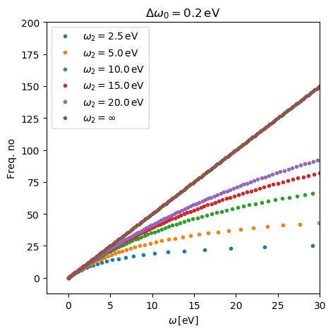
The dielectric function is evaluated on a non-linear frequency grid according to the formula

\[\omega_i = i \frac{\Delta\omega_0} {1 -(\sqrt2 - 1)\frac{\Delta\omega_0}{\omega_2} i}, i = 0, 1, ...,\]

The parameter \(\Delta\omega_0\) is the frequency spacing at \(\omega=0\) and \(\omega_2\) is the frequency where the spacing has increased to \(2\Delta\omega_0\). In general a lower value of \(\omega_2\) gives a more non- linear grid and less frequency points.

Below, the frequency grid is visualized for different values of \(\omega_2\). You can find the script for reproducing this figure here: plot_freq.py.

The parameters can be specified using keyword arguments:

df = DielectricFunction(
    ...,
    frequencies={'type': 'nonlinear', # frequency grid specification
                 'domega0: 0.05,      # eV. Default = 0.1 eV
                 'omega2': 5.0,       # eV. Default = 10.0 eV
                 'omegamax': 15.0})   # eV. Default is the maximum
                                      # difference between energy
                                      # eigenvalues

Setting omegamax manually is usually not advisable, however you might want it in cases where semi-core states are included where very large energy eigenvalue differences appear.

class gpaw.response.frequencies.FrequencyDescriptor(omega_w)

Frequency grid descriptor.

Parameters:

omega_w (ArrayLike1D) – Frequency grid in Hartree units.

static from_array_or_dict(input)

Create frequency-grid descriptor.

In case input is a list on frequencies (in eV) a FrequencyGridDescriptor instance is returned. Othervise a NonLinearFrequencyDescriptor instance is returned.

>>> from ase.units import Ha
>>> params = dict(type='nonlinear',
...               domega0=0.1,
...               omega2=10,
...               omegamax=50)
>>> wd = FrequencyDescriptor.from_array_or_dict(params)
>>> wd.omega_w[0:2] * Ha
array([0.        , 0.10041594])

class gpaw.response.frequencies.NonLinearFrequencyDescriptor(domega0, omega2, omegamax)

Non-linear frequency grid.

Units are Hartree. See Frequency grid.

Parameters:

• domega0 (float) – Frequency grid spacing for non-linear frequency grid at omega = 0.

• omega2 (float) – Frequency at which the non-linear frequency grid has doubled the spacing.

• omegamax (float) – The upper frequency bound for the non-linear frequency grid.

get_floor_index(o_m, safe=True)

Get closest index rounding down.

class gpaw.response.frequencies.FrequencyGridDescriptor(omega_w)

Frequency grid descriptor.

Parameters:

omega_w (ArrayLike1D) – Frequency grid in Hartree units.

get_index_range(lim1_m, lim2_m)

Get index range.

Example 1: Optical absorption of semiconductor: Bulk silicon

A simple startup

Here is a minimum script to get an absorption spectrum.

from ase.build import bulk
from gpaw import GPAW
from gpaw.response.df import DielectricFunction

# Part 1: Ground state calculation
atoms = bulk('Si', 'diamond', a=5.431)
calc = GPAW(mode='pw', kpts=(4, 4, 4))

atoms.calc = calc
atoms.get_potential_energy()  # ground state calculation is performed
calc.write('si.gpw', 'all')  # use 'all' option to write wavefunction

# Part 2 : Spectrum calculation
# DF: dielectric function object
# Ground state gpw file (with wavefunction) as input
df = DielectricFunction(
    calc='si.gpw',
    frequencies={'type': 'nonlinear',
                 'domega0': 0.05},  # using nonlinear frequency grid
    rate='eta')
# By default, a file called 'df.csv' is generated
df.get_dielectric_function()

This script takes less than one minute on a single cpu, and generates a file ‘df.csv’ containing the optical (\(\mathbf{q} = 0\)) dielectric function along the x-direction, which is the default direction. The file ‘df.csv’ contain five columns ordered as follows: \(\omega\) (eV), \(\mathrm{Re}(\epsilon_{\mathrm{NLF}})\), \(\mathrm{Im}(\epsilon_{\mathrm{NLF}})\), \(\mathrm{Re}(\epsilon_{\mathrm{LF}})\), \(\mathrm{Im}(\epsilon_{\mathrm{LF}})\) where \(\epsilon_{\mathrm{NLF}}\) and \(\epsilon_{\mathrm{LF}}\) is the result without and with local field effects, respectively.

For other directions you can specify the direction and filename like:

DielectricFunction.get_dielectric_function(...,
                                           direction='y',
                                           filename='filename.csv',
                                           ...)

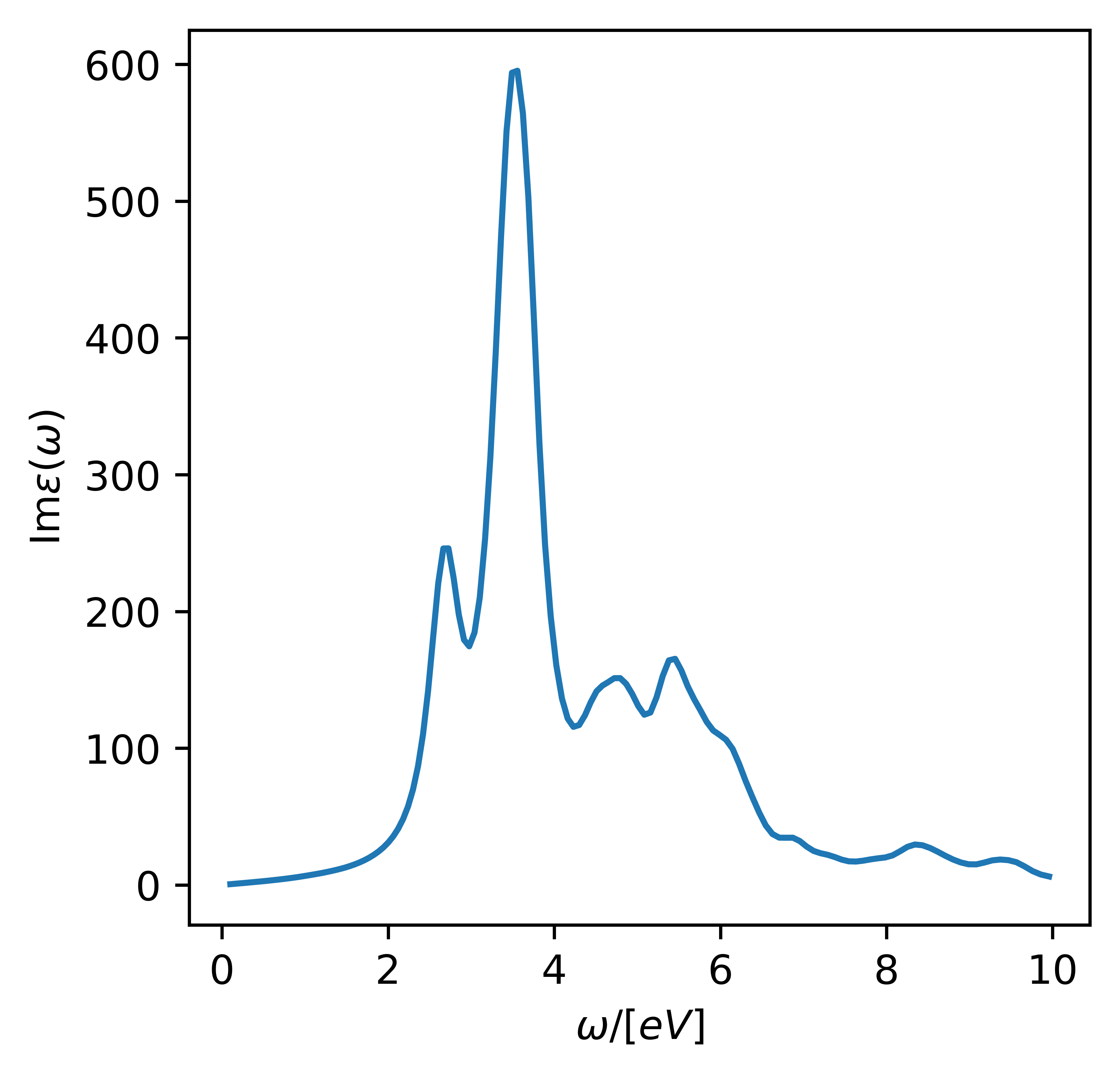
The absorption spectrum along the x-direction including local field effects can then be plotted using

# web-page: si_abs.png
import numpy as np
from math import pi
import matplotlib.pyplot as plt
from matplotlib import rc
rc('font', **{'family': 'sans-serif', 'sans-serif': ['Helvetica']})
# rc('text', usetex=True)
rc('figure', figsize=(4.0, 4.0), dpi=800)

data = np.loadtxt('df.csv', delimiter=',')

# Set plotting range
xmin = 0.1
xmax = 10.0
inds_w = (data[:, 0] >= xmin) & (data[:, 0] <= xmax)

plt.plot(data[inds_w, 0], 4 * pi * data[inds_w, 4])
plt.xlabel('$\\omega / [eV]$')
plt.ylabel('$\\mathrm{Im} \\epsilon(\\omega)$')
plt.savefig('si_abs.png', bbox_inches='tight')

The resulting figure is shown below. Note that there is significant absorption close to \(\omega=0\) because of the large default Fermi-smearing in GPAW. This will be dealt with in the following more realistic calculation.

More realistic calculation

To get a realistic silicon absorption spectrum and macroscopic dielectric constant, one needs to converge the calculations with respect to grid spacing, kpoints, number of bands, planewave cutoff energy and so on. Here is an example script: silicon_ABS.py. In the following, the script is split into different parts for illustration.

1. Ground state calculation

# Refer to G. Kresse, Phys. Rev. B 73, 045112 (2006)
# for comparison of macroscopic and microscopic dielectric constant
# and absorption peaks.
from pathlib import Path

from ase.build import bulk
from ase.parallel import paropen, world

from gpaw import GPAW, FermiDirac
from gpaw.response.df import DielectricFunction

# Ground state calculation
a = 5.431
atoms = bulk('Si', 'diamond', a=a)

calc = GPAW(mode='pw',
            kpts={'density': 5.0, 'gamma': True},
            parallel={'band': 1, 'domain': 1},
            xc='LDA',
            occupations=FermiDirac(0.001))  # use small FD smearing

atoms.calc = calc
atoms.get_potential_energy()  # get ground state density

# Restart Calculation with fixed density and dense kpoint sampling
calc = calc.fixed_density(
    kpts={'density': 15.0, 'gamma': False})  # dense kpoint sampling

calc.diagonalize_full_hamiltonian(nbands=70)  # diagonalize Hamiltonian
calc.write('si_large.gpw', 'all')  # write wavefunctions

In this script a normal ground state calculation is performed with coarse kpoint grid. The calculation is then restarted with a fixed density and the full hamiltonian is diagonalized exactly on a densely sampled kpoint grid. This is the preferred procedure of obtained the excited KS-states because it is in general difficult to converge the excited states using iterative solvers. A full diagonalization is more robust.

Note

For semiconductors, it is better to use either small Fermi-smearing in the ground state calculation:

from gpaw import FermiDirac
calc = GPAW(...
            occupations=FermiDirac(0.001),
            ...)

or larger ftol, which determines the threshold for transition in the dielectric function calculation (\(f_i - f_j > ftol\)), not shown in the example script):

df = DielectricFunction(...
                        ftol=1e-2,
                        ...)

2. Get absorption spectrum

# Getting absorption spectrum
df = DielectricFunction(calc='si_large.gpw',
                        eta=0.05,
                        frequencies={'type': 'nonlinear', 'domega0': 0.02},
                        ecut=150)
df.get_dielectric_function(filename='si_abs.csv')

Here eta is the broadening parameter of the calculation, and ecut is the local field effect cutoff included in the dielectric function.

3. Get macroscopic dielectric constant

The macroscopic dielectric constant is defined as the real part of dielectric function at \(\omega=0\). In the following script, only a single point at \(\omega=0\) is calculated without using the hilbert transform (which is only compatible with the non-linear frequency grid specification).

# Getting macroscopic constant
df = DielectricFunction(calc='si_large.gpw',
                        frequencies=[0.0],
                        hilbert=False,
                        eta=0.0001,
                        ecut=150,
                        )

epsNLF, epsLF = df.get_macroscopic_dielectric_constant()

# Make table
epsrefNLF = 14.08  # from [1] in top
epsrefLF = 12.66  # from [1] in top

with paropen('mac_eps.csv', 'w') as f:
    print(' , Without LFE, With LFE', file=f)
    print(f"{'GPAW-linear response'}, {epsNLF:.6f}, {epsLF:.6f}", file=f)
    print(f"{'[1]'}, {epsrefNLF:.6f}, {epsrefLF:.6f}", file=f)
    print(f"{'Exp.'}, {11.9:.6f}, {11.9:.6f}", file=f)

if world.rank == 0:
    Path('si_large.gpw').unlink()

In general, local field correction will reduce this value by 10-20%.

Result

The figure shown here is generated from script : silicon_ABS.py and plot_ABS.py. It takes 30 minutes with 16 cpus on Intel Xeon X5570 2.93GHz.

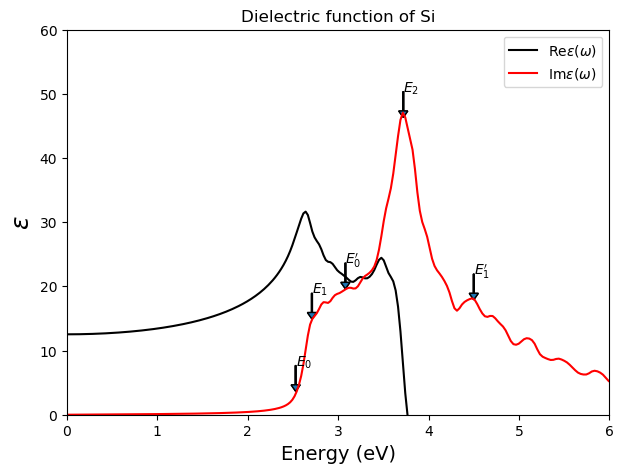
The arrows are data extracted from [1].

The calculated macroscopic dielectric constant can be seen in the table below and compare good with the values from [1]. The experimental value is 11.90. The larger theoretical value results from the fact that the ground state LDA (even GGA) calculation underestimates the bandgap.

	Without LFE	With LFE
GPAW-linear response	13.934931	12.532885
[1]	14.080000	12.660000
Exp.	11.900000	11.900000

Example 2: Electron energy loss spectra

Electron energy loss spectra (EELS) can be used to explore the plasmonic (collective electronic) excitations of an extended system. This is because the energy loss of a fast electron passing by a material is defined by

\[\mathrm{EELS} = -\mathrm{Im} \frac{1}{\epsilon(\mathbf{q}, \omega)}\]

and the plasmon frequency \(\omega_p\) is defined as \(\epsilon(\omega_p) \rightarrow 0\). It means that an external perturbation at this frequency, even infinitesimal, can generate a large collective electronic response.

A simple startup: bulk aluminum

Here is a minimum script to get an EELS spectrum.

from ase.build import bulk
from gpaw import GPAW
from gpaw.response.df import DielectricFunction

# Part 1: Ground state calculation
atoms = bulk('Al', 'fcc', a=4.043)  # generate fcc crystal structure
# GPAW calculator initialization:
k = 13
calc = GPAW(mode='pw', kpts=(k, k, k))

atoms.calc = calc
atoms.get_potential_energy()  # ground state calculation is performed
calc.write('Al.gpw', 'all')  # use 'all' option to write wavefunctions

# Part 2: Spectrum calculation
df = DielectricFunction(calc='Al.gpw')  # ground state gpw file as input

# Momentum transfer, must be the difference between two kpoints:
q_c = [1.0 / k, 0, 0]
df.get_eels_spectrum(q_c=q_c)  # by default, an 'eels.csv' file is generated

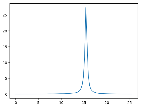
This script takes less than one minute on a single cpu and by default, generates a file ‘EELS.csv’. Then you can plot the file using

# web-page: aluminum_EELS.png
import numpy as np
import matplotlib.pyplot as plt

data = np.loadtxt('eels.csv', delimiter=',')
plt.plot(data[:, 0], data[:, 2])
plt.savefig('aluminum_EELS.png', bbox_inches='tight')
plt.show()

The three columns of this file correspond to energy (eV), EELS without and with local field correction, respectively. You will see a 15.9 eV peak. It comes from the bulk plasmon excitation of aluminum. You can explore the plasmon dispersion relation \(\omega_p(\mathbf{q})\) by tuning \(\mathbf{q}\) in the calculation above.

Note

The momentum transfer \(\mathbf{q}\) in an EELS calculation must be the difference between two kpoints! For example, if you have an kpts=(Nk1, Nk2, Nk3) Monkhorst-Pack k-sampling in the ground state calculation, you have to choose \(\mathbf{q} = \mathrm{np.array}([i/Nk1, j/Nk2, k/Nk3])\), where \(i, j, k\) are integers.

A more sophisticated example: graphite

Here is a more sophisticated example of calculating EELS of graphite with different \(\mathbf{q}\). You can also get the script here: graphite_EELS.py. The results (plot) are shown in the following section.

from math import sqrt
import numpy as np
from ase import Atoms
from ase.parallel import paropen
from gpaw import GPAW, FermiDirac, PW
from gpaw.response.df import DielectricFunction

# Part 1: Ground state calculation
a = 1.42
c = 3.355

# Generate graphite AB-stack structure:
atoms = Atoms('C4',
              scaled_positions=[(1 / 3.0, 1 / 3.0, 0),
                                (2 / 3.0, 2 / 3.0, 0),
                                (0, 0, 0.5),
                                (1 / 3.0, 1 / 3.0, 0.5)],
              pbc=(1, 1, 1),
              cell=[(sqrt(3) * a / 2, 3 / 2.0 * a, 0),
                    (-sqrt(3) * a / 2, 3 / 2.0 * a, 0),
                    (0, 0, 2 * c)])

# Part 2: Find ground state density and diagonalize full hamiltonian
calc = GPAW(mode=PW(500),
            kpts=(6, 6, 3),
            parallel={'domain': 1},
            # Use smaller Fermi-Dirac smearing to avoid intraband transitions:
            occupations=FermiDirac(0.05))

atoms.calc = calc
atoms.get_potential_energy()

calc = calc.fixed_density(kpts=(20, 20, 7))

# The result should also be converged with respect to bands:
calc.diagonalize_full_hamiltonian(nbands=60)
calc.write('graphite.gpw', 'all')

# Part 2: Spectra calculations
f = paropen('graphite_q_list', 'w')  # write q

for i in range(1, 6):  # loop over different q
    df = DielectricFunction(calc='graphite.gpw',
                            frequencies={'type': 'nonlinear',
                                         'domega0': 0.01},
                            eta=0.2,  # Broadening parameter.
                            ecut=100,
                            # write different output for different q:
                            txt='out_df_%d.txt' % i)

    q_c = [i / 20.0, 0.0, 0.0]  # Gamma - M excitation

    df.get_eels_spectrum(q_c=q_c, filename='graphite_EELS_%d' % i)

    # Calculate cartesian momentum vector:
    cell_cv = atoms.get_cell()
    bcell_cv = 2 * np.pi * np.linalg.inv(cell_cv).T
    q_v = np.dot(q_c, bcell_cv)
    print(sqrt(np.inner(q_v, q_v)), file=f)

f.close()

Results on graphite

The figure shown here is generated from script: graphite_EELS.py and plot_EELS.py

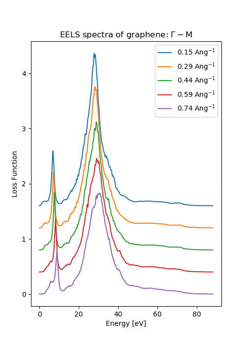
One can compare the results with literature [2].

Example 3: Tetrahedron integration (experimental)

The k-point integral needed for the calculation of the density response function, is typically performed using a simple summation of individual k-points. By setting the integration mode to ‘tetrahedron integration’ the kpoint integral is calculated by interpolating density matrix elements and eigenvalues. This typically means that fewer k-points are needed for convergence.

The combination of using the tetrahedron method and reducing the kpoint integral using crystal symmetries means that it is necessary to be careful with the kpoint sampling which should span the whole irreducible zone. Luckily, bztools.py provides the tool to generate such an k-point sampling autimatically:

from gpaw.bztools import find_high_symmetry_monkhorst_pack
kpts = find_high_symmetry_monkhorst_pack(
    'gs.gpw',  # Path to ground state .gpw file
    density=20.0)  # The required minimum density

Bulk TaS₂

As an example, lets calculate the optical properties of a well-known layered material, namely, the transition metal dichalcogenide (TMD) 2H-TaS₂. We set the structure and find the ground state density with (find the full script here tas2_dielectric_function.py, takes about 10 mins on 8 cores.)

# web-page: tas2_eps.png
from ase import Atoms
from ase.lattice.hexagonal import Hexagonal
import matplotlib.pyplot as plt

from gpaw import GPAW, PW, FermiDirac
from gpaw.response.df import DielectricFunction
from gpaw.mpi import world
from gpaw.bztools import find_high_symmetry_monkhorst_pack

# 1) Ground-state.

a = 3.314
c = 12.1

cell = Hexagonal(symbol='Ta', latticeconstant={'a': a, 'c': c}).get_cell()
atoms = Atoms(symbols='TaS2TaS2', cell=cell, pbc=(1, 1, 1),
              scaled_positions=[(0, 0, 1 / 4),
                                (2 / 3, 1 / 3, 1 / 8),
                                (2 / 3, 1 / 3, 3 / 8),
                                (0, 0, 3 / 4),
                                (-2 / 3, -1 / 3, 5 / 8),
                                (-2 / 3, -1 / 3, 7 / 8)])

calc = GPAW(mode=PW(600),
            xc='PBE',
            occupations=FermiDirac(width=0.01),
            kpts={'density': 5})

atoms.calc = calc
atoms.get_potential_energy()
calc.write('TaS2-gs.gpw')

The next step is to calculate the unoccupied bands

kpts = find_high_symmetry_monkhorst_pack('TaS2-gs.gpw', density=5.0)

responseGS = GPAW('TaS2-gs.gpw').fixed_density(
    kpts=kpts,
    parallel={'band': 1},
    nbands=60,
    convergence={'bands': 50})

responseGS.get_potential_energy()
responseGS.write('TaS2-gsresponse.gpw', 'all')

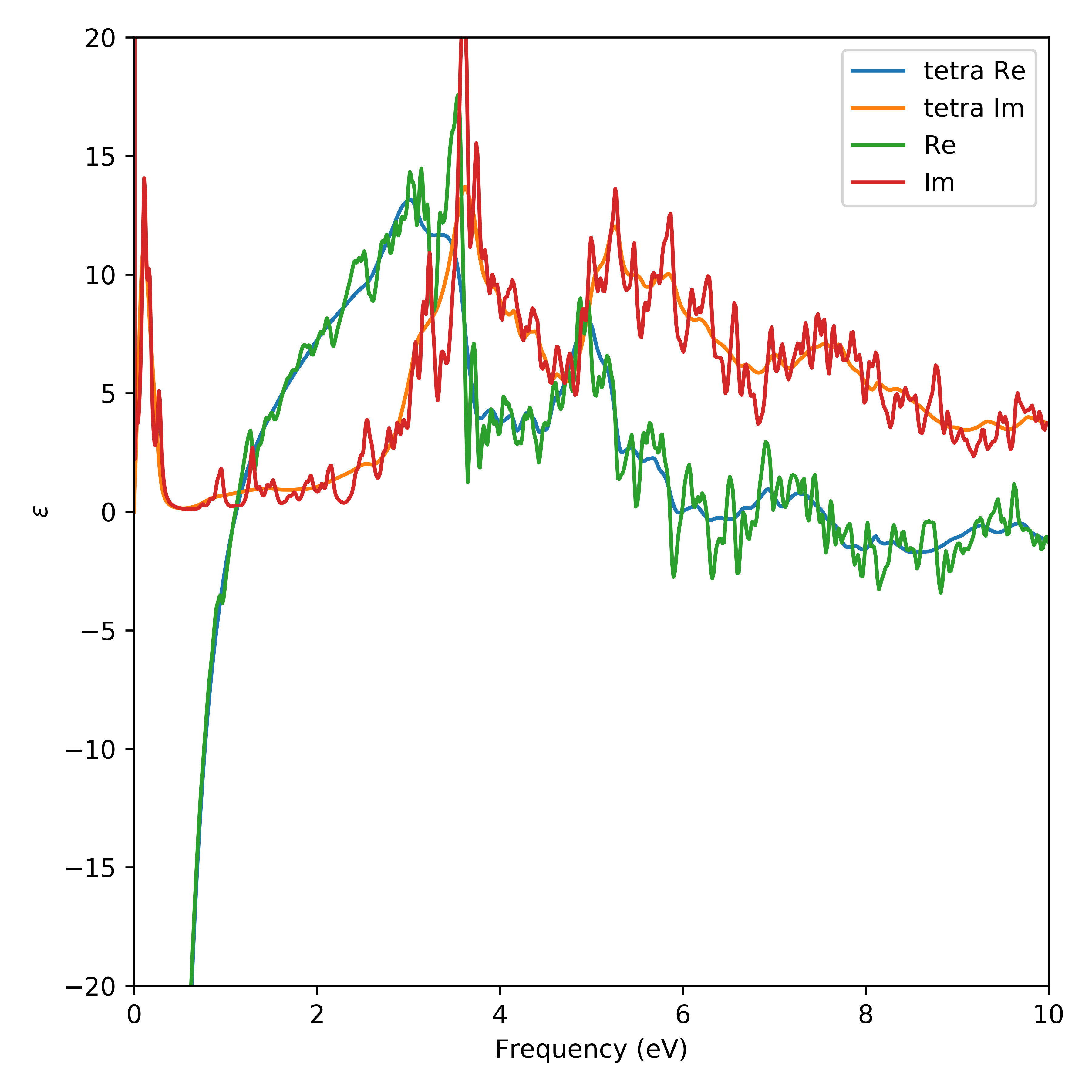
Lets compare the result of the tetrahedron method with the point sampling method for broadening of eta=25 meV.

df = DielectricFunction(
    'TaS2-gsresponse.gpw',
    eta=25e-3,
    rate='eta',
    frequencies={'type': 'nonlinear', 'domega0': 0.01},
    integrationmode='tetrahedron integration')

df1tetra_w, df2tetra_w = df.get_dielectric_function(direction='x')

df = DielectricFunction(
    'TaS2-gsresponse.gpw',
    eta=25e-3,
    rate='eta',
    frequencies={'type': 'nonlinear', 'domega0': 0.01})
df1_w, df2_w = df.get_dielectric_function(direction='x')
omega_w = df.get_frequencies()

if world.rank == 0:
    plt.figure(figsize=(6, 6))
    plt.plot(omega_w, df2tetra_w.real, label='tetra Re')
    plt.plot(omega_w, df2tetra_w.imag, label='tetra Im')
    plt.plot(omega_w, df2_w.real, label='Re')
    plt.plot(omega_w, df2_w.imag, label='Im')
    plt.xlabel('Frequency (eV)')
    plt.ylabel('$\\varepsilon$')
    plt.xlim(0, 10)
    plt.ylim(-20, 20)
    plt.legend()
    plt.tight_layout()
    plt.savefig('tas2_eps.png', dpi=600)
#    plt.show()

The result of which is shown below. Comparing the methods shows that the calculated dielectric function is much more well behaved when calculated using the tetrahedron method.

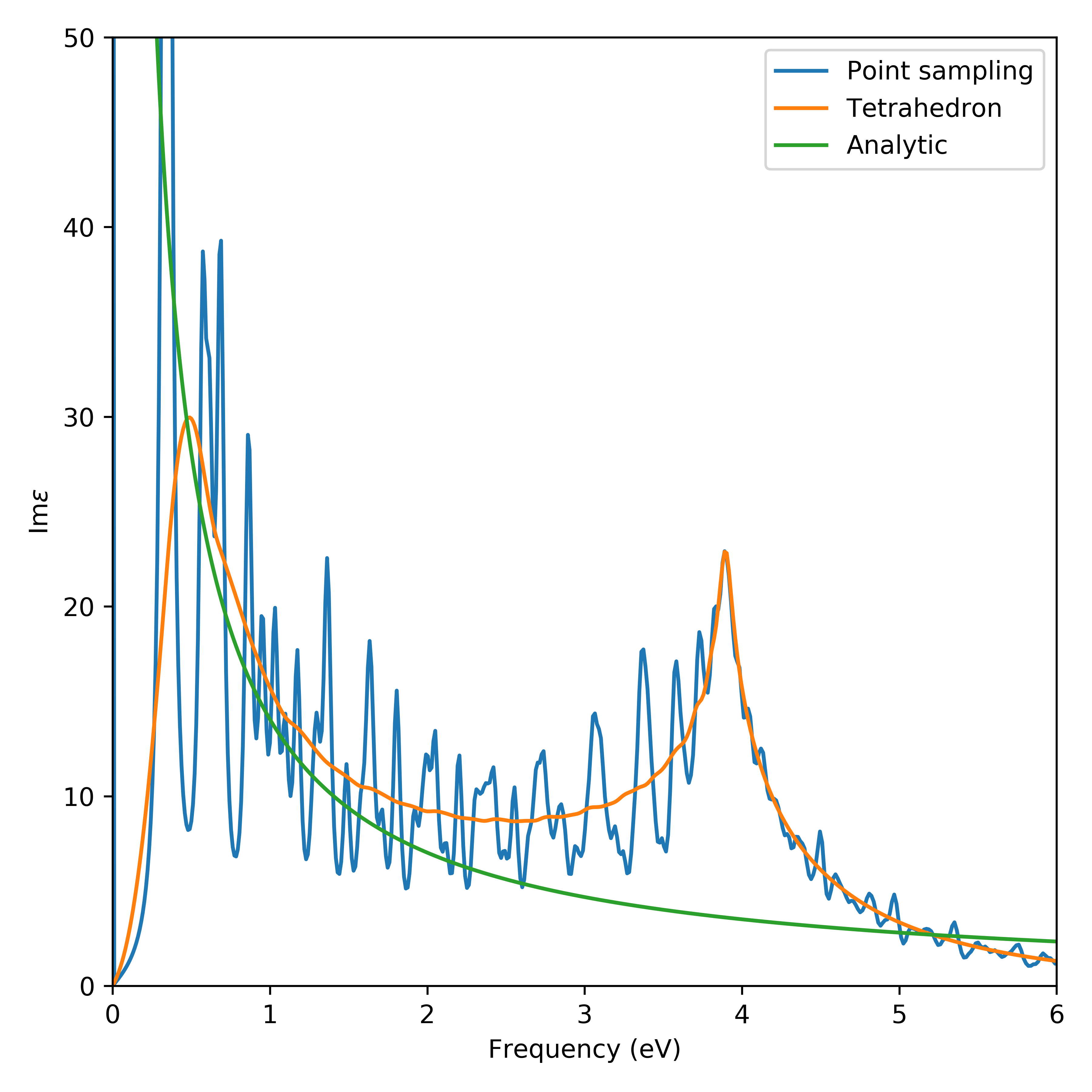
Graphene

Graphene represents a material which is particularly difficult to converge with respect to the number of k-points. This property originates from its semi-metallic nature and vanishing density of states at the fermi-level which make the calculated properties sensitive to the k-point distribution in the vicinity of the Dirac point. Since the macroscopic dielectric function is not well-defined for two-dimensional systems we will focus on calculating the dielectric function an artificial structure of graphite with double the out-of-plane lattice constant. This should make its properties similar to graphene. It is well known that graphene has a sheet conductance of \(\sigma_s=\frac{e^2}{4\hbar}\) so, if the individual graphite layers behave as ideal graphene, the optical properties of the structure should be determined by

\[\varepsilon = 1 + \frac{4 \pi i}{\omega d} \sigma_s\]

where \(d=3.22\) Å is the thickness of graphene. Below we show the calculated dielectic function (graphene_dielectric_function.py) for a minimum k-point density of 30 Å\(^{-1}\) corresponding to a kpoint sampling of size (90, 90, 1) and room temperatur broadening eta = 25 meV. It is clear that the properties are well converged for large frequencies using the tetrahedron method. For smaller frequencies the tetrahedron method fares comparably but convergence is tough for frequencies below 0.5 eV where the absorption spectrum goes to zero. This behaviour is due to the partially occupied Dirac point which sensitively effects the integrand of the density response function.

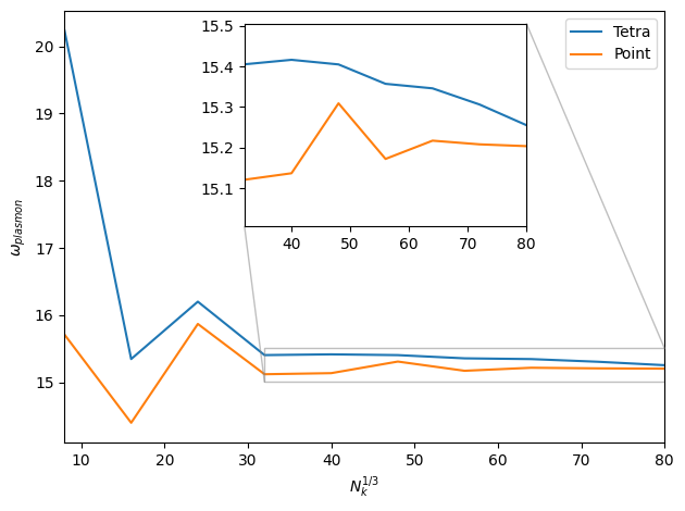
k-point convergence comparison

Elemental aluminium is another material which can be difficult to converge with respect to the number of k-points. This is due to the Fermi surface of the metal penetrating the surface of the first Brilluoin zone. This means that the fermi surface has to be finely resolved when calculating ´q = 0´ EELS spectra. The EELS spectrum of Al shows a clear plasmonic resonsance and below we show the k-point convergence of the plasmon frequency. We compare the tetrahedron integration described here with the default point integration method. The dielectric function is calculated for all varying k-samplings (al-plasmon-peak.py) using ´Gamma´-centered Monkhorst-Pack k-point grids with a multiple of 8 points along each axis to ensure sampling of high-symmetry k-points. We see that both methods converge to the same value.

Notes on the implementation of the tetrahedron method

The tetrahedron method is still in an experimental phase which means that the user should check the results against the results obtained with point integration. The method is based on the paper of [3] whom provide analytical expressions for the response function integration with interpolated eigenvalues and matrix elements.

In other implementations of the tetrahedron integration method, the division of the BZ into tetrahedras has been performed using a recursive scheme. In our implementation we use the external library scipy.spatial which provide the Delaunay() class to calculate Delaunay triangulated k-point grids from the ground state k-point grid. Delaunay triangulated grids do necessarily give a good division of the Brillouin zone into tetrahedras and particularly for homogeneously spaced k-point grids (such as a Monkhorst Pack) grid many ill-defined tetrahedrons may be created. Such tetrahedrons are however easily filtered away by removing tetrahedrons with very small volumes.

• Suggested performance enhancement: TetrahedronDescriptor(kpts, simplices=None) Factor out the creation of tetrahedras to make it possible to use user-defined tetrahedras. Such an object could inherit from the Delaunay() class.

Additionally, this library provides a k-dimensional tree implementation cKDTree() which is used to efficiently identify k-points in the Brillouin zone. For finite \(\mathbf{q}\) it is still necessary for the kpoint grid to be uniform. In the optical limit where \(\mathbf{q}=0\), however, it is possible to use non-uniform k-point grids which can aid a faster convergence, especially for materials such as graphene.

When using the tetrahedron integration method, the plasmafrequency is calculated at \(T=0\) where the expression reduces an integral over the Fermi surface. The interband transitions are calculated using the temperature of the ground state calculation. The occupation factors are included as modifications to the matrix elements as \(\sqrt{f_n - f_m} \langle \psi_m|\nabla |\psi_n \rangle\)

• Suggested performance enhancement: Take advantage of the analytical dependence of the occupation numbers to treat partially occupied bands more accurately. This is expected to improve the convergence of the optical properties of graphene for low frequencies.

The entirety of the tetrahedron integration code is written in Python except for the calculation of the algebraic expression for the response function integration of a single tetrahedron for which the Python overhead is significant. The algebraic expression are therefore evaluated in C.

Technical details:

There are few points about the implementation that we emphasize:

• The code is parallelized over kpoints and occupied bands. The parallelization over occupied bands makes it straight-forward to utilize efficient BLAS libraries to sum un-occupied bands.

• The code employs the Hilbert transform in which the spectral function for the density-density response function is calculated before calculating the full density response. This speeds up the code significantly for calculations with a lot of frequencies.

• The non-linear frequency grid employed in the calculations is motivated by the fact that when using the Hilbert transform the real part of the dielectric function converges slowly with the upper bound of the frequency grid. Refer to Linear dielectric response of an extended system: theory for the details on the Hilbert transform.

Drude phenomenological scattering rate

A phenomenological scattering rate can be introduced using the rate parameter in the optical limit. By default this is zero but can be set by using:

df = DielectricFunction(...
                        rate=0.1,
                        ...)

to set a scattering rate of 0.1 eV. If rate=’eta’ then the code with use the specified eta parameter. Note that the implementation of the rate parameter differs from some literature by a factor of 2 for consistency with the linear response formalism. In practice the Drude rate is implemented as

\[\frac{\omega_\mathrm{p}^2}{(\omega + i\gamma)^2}\]

where \(\gamma\) is the rate parameter.

Useful tips

Use --dry-run option to get an overview of a calculation (especially useful for heavy calculations!):

$ gpaw python --dry-run=8 filename.py

Note

But be careful ! LCAO mode calculation results in unreliable unoccupied states above vacuum energy.

It’s important to converge the results with respect to:

nbands,
nkpt (number of kpoints in gs calc.),
eta,
ecut,
ftol,
omegamax (the maximum energy, be careful if hilbert transform is used)
domega0 (the energy spacing, if there is)
vacuum (if there is)

Parameters

keyword	type	default value	description
calc	str	None	gpw filename (with ‘all’ option when writing the gpw file)
name	str	None	If specified the chi matrix is saved to chi+qx+qy+qz.pckl where qx, qy, qz is the wave-vector components in reduced coordinates.
frequencies	numpy.ndarray	None	Energies for spectrum. If left unspecified the frequency grid will be non-linear. Ex: numpy.linspace(0,20,201)
domega0	float	0.1	\(\Delta\omega_0\) for non-linear frequency grid.
omega2	float	10.0 (eV)	\(\omega_2\) for non-linear frequencygrid.
omegamax	float	Maximum energy eigenvalue difference.	Maximum frequency.
ecut	float	10 (eV)	Planewave energy cutoff. Determines the size of dielectric matrix.
eta	float	0.2 (eV)	Broadening parameter.
ftol	float	1e-6	The threshold for transition: \(f_{ik} - f_{jk} > ftol\)
txt	str	stdout	Output filename.
hilbert	bool	True	Switch for hilbert transform.
nbands	int	nbands from gs calc	Number of bands from gs calc to include.
rate	float or str	0.0 (eV)	Phenomenological Drude scattering rate. If rate=”eta” then use “eta”. Note that this may differ by a factor of 2 for some definitions of the Drude scattering rate. See the section on Drude scattering rate.

Details of the DF object

class gpaw.response.df.DielectricFunction(calc, *, frequencies=None, ecut=50, hilbert=True, nbands=None, eta=0.2, intraband=True, nblocks=1, world=MPIComm(size=1, rank=0), txt=<_io.TextIOWrapper name='<stdout>' mode='w' encoding='utf-8'>, truncation=None, disable_point_group=False, disable_time_reversal=False, integrationmode=None, rate=0.0, eshift=0.0)

This class defines dielectric function related physical quantities.

Creates a DielectricFunction object.

calc: str

The ground-state calculation file that the linear response calculation is based on.

frequencies:

Input parameters for frequency_grid. Can be an array of frequencies to evaluate the response function at or dictionary of parameters for build-in nonlinear grid (see Frequency grid).

ecut: float

Plane-wave cut-off.

hilbert: bool

Use hilbert transform.

nbands: int

Number of bands from calculation.

eta: float

Broadening parameter.

intraband: bool

Include intraband transitions.

world: comm

mpi communicator.

nblocks: int

Split matrices in nblocks blocks and distribute them G-vectors or frequencies over processes.

txt: str

Output file.

truncation: str or None

None for no truncation. ‘2D’ for standard analytical truncation scheme. Non-periodic directions are determined from k-point grid

eshift: float

Shift unoccupied bands

get_dielectric_function(*args, **kwargs)

…

get_eels_spectrum(*args, **kwargs)

…

get_macroscopic_dielectric_constant(xc='RPA', direction='x', q_v=None)

Calculate macroscopic dielectric constant.

Returns eM_NLFC and eM_LFC.

Macroscopic dielectric constant is defined as the real part of dielectric function at w=0.

Parameters:

eM_LFC: float

Dielectric constant without local field correction. (RPA, ALDA)

eM2_NLFC: float

Dielectric constant with local field correction.

[1] (1,2)

M. Gajdoš, K. Hummer, G. Kresse, J. Furthmüller and F. Bechstedt, Linear optical properties in the projected-augmented wave methodology, Phys. Rev. B 73, 045112 (2006).

[2]

A. G. Marinopoulos, L. Reining, A. Rubio and V. Olevano, Ab initio study of the optical absorption and wave-vector-dependent dielectric response of graphite, Phys. Rev. B 69, 245419 (2004).

[3]

1. MacDonald, A. H., Vosko, S. H. & Coleridge, P. T., Extensions of the tetrahedron method for evaluating spectral properties of solids. J. Phys. C Solid State Phys. 12, 2991–3002 (1979).