Local Orbitals
In this section we will describe how to obtain the Local Orbitals (LOs). The details of the theory are described in Ref. [1]. The starting point is a DFT calculation in LCAO mode:
from gpaw.local_orbitals import LocalOrbitals
calc = GPAW(mode='lcao', ...)
los = LocalOrbitals(calc)
The local orbitals are obtained from a sub-diagonalization of the LCAO Hamiltonian.
A sub-diagonalization is essentially a rotation that brings the
Hamiltonian in a form where some blocks are diagonal matrices.
Each block should include all Atomic Orbitals of a given atom.
This tranformation can be performed with the subdiagonalization method:
los.subdiagonalize(symbols: Array1D = None, blocks: list[list] = None, groupby: str = 'energy')
The blocks can be specified with one of the two keyword arguments:
symbols: Element or elements to sub-diagonalize, optional.Automatically constructs the blocks for the specified element or elements.
blocks: Blocks to sub-diagonalize, optional.Directly provides the blocks in the form of a list of orbital indices, e.g. [[3,4,5],[6,7..]..].
Once the Hamiltonian is sub-diagonalized, the method tries to group the obtained LOs by symmetry:
groupby: Grouping criteria.energy : Groups the LOs by energy
symmetry : Groups the LOs by spatial symmetry and energy
It is possible to fine-tune the grouping after a sub-diagonalization with the following method:
los.groupby(method: str = 'energy', decimals: int = 1, cutoff: float = 0.9),
decimals: Round energies to the given number of decimalsGroups the LOs with an energy equivalent up to the given number of decimals.
cutoff: Cutoff spatial overlap, (0,1]Groups the LOs with a spatial overlap larger than the given cutoff value.
Next, we construct a low-energy model from a subset of LOs and/or AOs:
los.take_model(indices: Array1D = None, minimal: bool = True, cutoff: float = 1e-3, ortho: bool = False)
indices: Orbitals to include in the low-energy model, optionalExplicitely lists the orbital indices in the sub-diagonalized Hamiltonian. When left unspecified, the method will automacally select the orbitals in each
blockwith the energy closest to the Fermi level. We call thisminimalmodel.minimal: Limit the selection to the givenindicesTrue : Default value.
False : Extend the minimal model with the groups of LOs connecting to the minimal model with at least one matrix element in the Hamiltonian larger than
cutoff.
otho: Orthogonalize the low-energy modelOrthogonalizes the orbitals in the low-energy model. We advise to use this flag only for minimal models.
Local Orbitals in benzene molecule
As a first example we generate the local orbitals (LOs) of an
isolated benzene molecule C6H6.py.
benzene = molecule('C6H6', vacuum=5)
# LCAO calculation
calc = GPAW(mode='lcao', xc='LDA', basis='szp(dzp)', txt=None)
calc.atoms = benzene
calc.get_potential_energy()
# LCAO wrapper
lcao = LCAOwrap(calc)
# Construct a LocalOrbital Object
los = LocalOrbitals(calc)
# Subdiagonalize carbon atoms and group by energy.
los.subdiagonalize('C', groupby='energy')
# Groups of LOs are stored in a dictionary >>> los.groups
# Dump pz-type LOs in cube format
fig = los.plot_group(-6.9)
fig.savefig('C6H6_pzLOs.png', dpi=300, bbox_inches='tight')
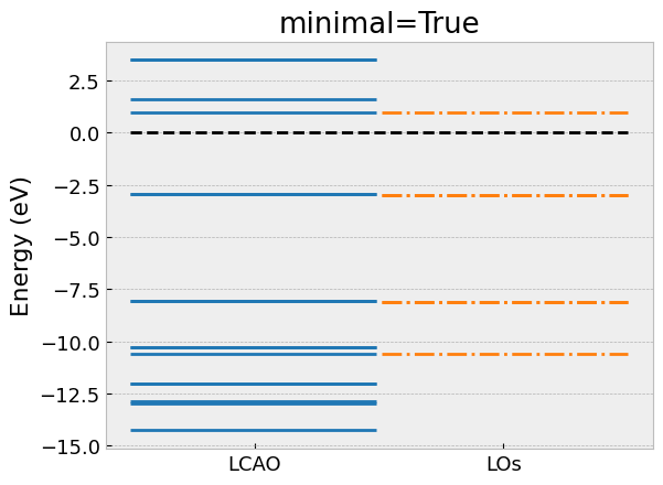
# Take minimal model
los.take_model(minimal=True)
# Get the size of the model >>> len(los.model)
# Assert that the Hamiltonian has the same
# dimensions >> los.get_hamiltonian().shape
# Assert model indeed conicides with pz-type LOs
assert los.indices == los.groups[-6.9]
# Compare eigenvalues with LCAO
compare_eigvals(lcao, los, "C6H6_minimal.png", "minimal=True")
# Extend with groups of LOs that overlap with the minimal model
los.take_model(minimal=False)
# Get the size of the model >>> len(los.model)
# Assert model is extended with other groups.
assert los.indices == (los.groups[-6.9] + los.groups[20.2] + los.groups[21.6])
# Compare eigenvalues with LCAO
compare_eigvals(lcao, los, "C6H6_extended.png", "minimal=False")
Here, we have omitted the import statements and the declaration of
the compare_eigvals helper function to visually compare the
eigenvalues of the low-energy model with the full LCAO calculation as horizontal lines.

Isourfaces of local orbitals with pz-character.

Local Orbitals in graphene nanoribbon
As a second example we generate the local orbitals (LOs) of a
graphene nanoribbon C4H2.py.
gnr = graphene_nanoribbon(2, 1, type='zigzag', saturated=True,
C_H=1.1, C_C=1.4, vacuum=5.0)
# LCAO calculation
calc = GPAW(mode='lcao',
xc='LDA',
basis='szp(dzp)',
txt=None,
kpts={'size': (1, 1, 11),
'gamma': True},
symmetry={'point_group': False,
'time_reversal': True})
calc.atoms = gnr
calc.get_potential_energy()
# Start post-process
tb = TightBinding(calc.atoms, calc)
# Construct a LocalOrbital Object
los = LocalOrbitals(calc)
# Subdiagonalize carbon atoms and group by symmetry and energy.
los.subdiagonalize('C', groupby='symmetry')
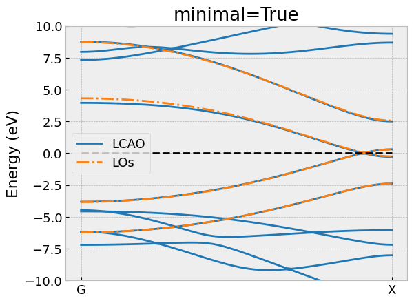
# Take minimal model
los.take_model(minimal=True)
# Compare the bandstructure of the effective model and compare it with LCAO
compare_bandstructure(tb, los, "C4H2_minimal.png", "minimal=True")
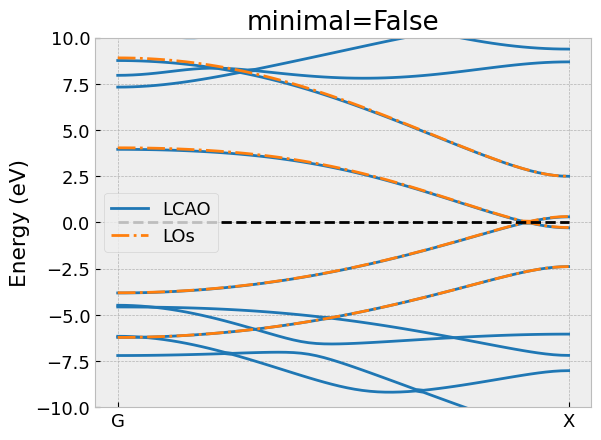
# Extend with groups of LOs that overlap with the minimal model
los.take_model(minimal=False)
# Compare the bandstructure of the effective model and compare it with LCAO
compare_bandstructure(tb, los, "C4H2_extended.png", "minimal=False")
Again, we have omitted the import statements and the declaration of
the compare_bandstructure helper function to compare the
bands of the low-energy model with the full LCAO calculation.