Induced density oscillations and electric near field from TDDFT
Calculating Fourier transform of the density oscillation at the resonant frequencies of a systems is a great way of analyzing the excitations. Induced density oscillations and the resulting electric near field can be calculated for finite systems from Time-propagation TDDFT or Linear response TDDFT (Casida’s equation).
For details of the implementation, see Ref. [1].
Time-propagation TDDFT
See Time-propagation TDDFT for instructions how to use time-propagation TDDFT.
Within time-propagation TDDFT, the induced density is obtained as an on-the-fly Fourier transform. A restriction of this iterative approach is that the frequencies of interest must be given at initialization, that is, before time propagation.
Example code for time-propagation calculation
from ase import Atoms
from gpaw import GPAW
from gpaw.tddft import TDDFT, DipoleMomentWriter, RestartFileWriter
from gpaw.inducedfield.inducedfield_tddft import TDDFTInducedField

# Na2 cluster
atoms = Atoms(symbols='Na2',
              positions=[(0, 0, 0), (3.0, 0, 0)],
              pbc=False)
atoms.center(vacuum=6.0)

# Standard ground state calculation
calc = GPAW(mode='fd', nbands=2, h=0.4, setups={'Na': '1'},
            symmetry={'point_group': False})
atoms.calc = calc
energy = atoms.get_potential_energy()
calc.write('na2_gs.gpw', mode='all')

# Standard time-propagation initialization
time_step = 10.0
iterations = 3000
kick_strength = [1.0e-3, 0.0, 0.0]
td_calc = TDDFT('na2_gs.gpw')
DipoleMomentWriter(td_calc, 'na2_td_dm.dat')
RestartFileWriter(td_calc, 'na2_td.gpw')

# Create and attach InducedField object
frequencies = [1.0, 2.08]     # Frequencies of interest in eV
folding = 'Gauss'             # Folding function
width = 0.1                   # Line width for folding in eV
ind = TDDFTInducedField(paw=td_calc,
                        frequencies=frequencies,
                        folding=folding,
                        width=width,
                        restart_file='na2_td.ind')

# Propagate as usual
td_calc.absorption_kick(kick_strength=kick_strength)
td_calc.propagate(time_step, iterations)

# Save TDDFT and InducedField objects
td_calc.write('na2_td.gpw', mode='all')
ind.write('na2_td.ind')
Example code for continuing time-propagation
from gpaw.tddft import TDDFT, DipoleMomentWriter, RestartFileWriter
from gpaw.inducedfield.inducedfield_tddft import TDDFTInducedField

# Load TDDFT object
td_calc = TDDFT('na2_td.gpw')
DipoleMomentWriter(td_calc, 'na2_td_dm.dat')
RestartFileWriter(td_calc, 'na2_td.gpw')

# Load and attach InducedField object
ind = TDDFTInducedField(filename='na2_td.ind',
                        paw=td_calc,
                        restart_file='na2_td.ind')

# Continue propagation as usual
time_step = 20.0
iterations = 250
td_calc.propagate(time_step, iterations)

# Save TDDFT and InducedField objects
td_calc.write('na2_td.gpw', mode='all')
ind.write('na2_td.ind')
Induced electric potential and near field are calculated after time-propagation as follows:
from gpaw.tddft import TDDFT, photoabsorption_spectrum
from gpaw.inducedfield.inducedfield_tddft import TDDFTInducedField

# Calculate photoabsorption spectrum as usual
folding = 'Gauss'
width = 0.1
e_min = 0.0
e_max = 4.0
photoabsorption_spectrum('na2_td_dm.dat', 'na2_td_spectrum_x.dat',
                         folding=folding, width=width,
                         e_min=e_min, e_max=e_max, delta_e=1e-2)

# Load TDDFT object
td_calc = TDDFT('na2_td.gpw')

# Load InducedField object
ind = TDDFTInducedField(filename='na2_td.ind',
                        paw=td_calc)

# Calculate induced electric field
ind.calculate_induced_field(gridrefinement=2, from_density='comp')

# Save induced electric field
ind.write('na2_td_field.ind', mode='all')
Plotting example (run in serial mode, i.e., with one process)
# web-page: na2_td_Ffe.png, na2_td_Frho.png, na2_td_Fphi.png
from gpaw.mpi import world
import numpy as np
import matplotlib.pyplot as plt
from gpaw.inducedfield.inducedfield_base import BaseInducedField
from gpaw.tddft.units import aufrequency_to_eV
assert world.size == 1, 'Script should be run in serial mode (one process).'
# Helper function
def do_plot(d_g, ng, box, atoms):
# Take slice of data array
d_yx = d_g[:, ng[1] // 2, :]
y = np.linspace(0, box[0], ng[0])
ylabel = u'x / Å'
x = np.linspace(0, box[2], ng[2])
xlabel = u'z / Å'
# Plot
plt.figure()
ax = plt.subplot(1, 1, 1)
X, Y = np.meshgrid(x, y)
plt.contourf(X, Y, d_yx, 40)
plt.colorbar()
for atom in atoms:
pos = atom.position
plt.scatter(pos[2], pos[0], s=50, c='k', marker='o')
plt.xlabel(xlabel)
plt.ylabel(ylabel)
plt.xlim([x[0], x[-1]])
plt.ylim([y[0], y[-1]])
ax.set_aspect('equal')
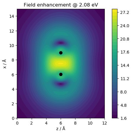
# Read InducedField object
ind = BaseInducedField('na2_td_field.ind', readmode='all')
# Choose array
w = 1 # Frequency index
freq = ind.omega_w[w] * aufrequency_to_eV # Frequency
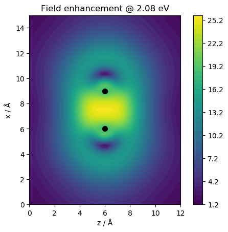
box = np.diag(ind.atoms.get_cell()) # Calculation box
d_g = ind.Ffe_wg[w] # Data array
ng = d_g.shape # Size of grid
atoms = ind.atoms # Atoms
do_plot(d_g, ng, box, atoms)
plt.title(f'Field enhancement @ {freq:.2f} eV')
plt.savefig('na2_td_Ffe.png', bbox_inches='tight')
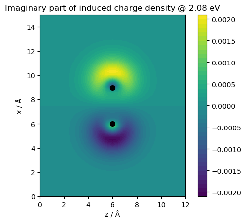
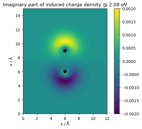
# Imaginary part of density
d_g = ind.Frho_wg[w].imag
ng = d_g.shape
do_plot(d_g, ng, box, atoms)
plt.title(f'Imaginary part of induced charge density @ {freq:.2f} eV')
plt.savefig('na2_td_Frho.png', bbox_inches='tight')
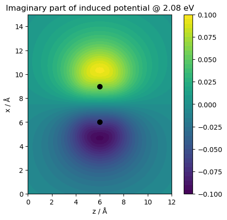
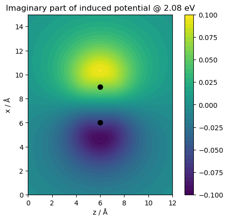
# Imaginary part of potential
d_g = ind.Fphi_wg[w].imag
ng = d_g.shape
do_plot(d_g, ng, box, atoms)
plt.title(f'Imaginary part of induced potential @ {freq:.2f} eV')
plt.savefig('na2_td_Fphi.png', bbox_inches='tight')
TODO: notes about AE/comp corrections, extending grid
Linear response TDDFT (Casida’s equation)
See Linear response TDDFT for instructions how to use linear response TDDFT.
Example code for linear response calculation
from ase import Atoms
from gpaw import GPAW
from gpaw.lrtddft import LrTDDFT

# Na2 cluster
atoms = Atoms(symbols='Na2',
              positions=[(0, 0, 0), (3.0, 0, 0)],
              pbc=False)
atoms.center(vacuum=6.0)

# Standard ground state calculation with empty states
calc = GPAW(mode='fd', nbands=100, h=0.4, setups={'Na': '1'})
atoms.calc = calc
energy = atoms.get_potential_energy()

calc = calc.fixed_density(
    convergence={'bands': 90})
calc.write('na2_gs_casida.gpw', mode='all')

# Standard Casida calculation
calc = GPAW('na2_gs_casida.gpw')
istart = 0
jend = 90
lr = LrTDDFT(calc, xc='LDA', restrict={'istart': istart, 'jend': jend})
lr.diagonalize()
lr.write('na2_lr.dat.gz')
Induced electric potential and near field are calculated as post-processing step as follows:
from gpaw import GPAW
from gpaw.lrtddft import LrTDDFT, photoabsorption_spectrum
from gpaw.inducedfield.inducedfield_lrtddft import LrTDDFTInducedField

# Load LrTDDFT object
lr = LrTDDFT.read('na2_lr.dat.gz')

# Calculate photoabsorption spectrum as usual
folding = 'Gauss'
width = 0.1
e_min = 0.0
e_max = 4.0
photoabsorption_spectrum(lr, 'na2_casida_spectrum.dat',
                         folding=folding, width=width,
                         e_min=e_min, e_max=e_max, delta_e=1e-2)

# Load GPAW object
calc = GPAW('na2_gs_casida.gpw')

# Calculate induced field
frequencies = [1.0, 2.08]     # Frequencies of interest in eV
folding = 'Gauss'             # Folding function
width = 0.1                   # Line width for folding in eV
kickdir = 0                   # Kick field direction 0, 1, 2 for x, y, z
ind = LrTDDFTInducedField(paw=calc,
                          lr=lr,
                          frequencies=frequencies,
                          folding=folding,
                          width=width,
                          kickdir=kickdir)
ind.calculate_induced_field(gridrefinement=2, from_density='comp')
ind.write('na2_casida_field.ind', mode='field')
Plotting example (same as in time propagation)
# web-page: na2_casida_Ffe.png, na2_casida_Frho.png, na2_casida_Fphi.png
from gpaw.mpi import world

import numpy as np
import matplotlib.pyplot as plt

from gpaw.inducedfield.inducedfield_base import BaseInducedField
from gpaw.tddft.units import aufrequency_to_eV

assert world.size == 1, 'Script should be run in serial mode (one process).'


# Helper function
def do_plot(d_g, ng, box, atoms):
    # Take slice of data array
    d_yx = d_g[:, ng[1] // 2, :]
    y = np.linspace(0, box[0], ng[0])
    ylabel = u'x / Å'
    x = np.linspace(0, box[2], ng[2])
    xlabel = u'z / Å'

    # Plot
    plt.figure()
    ax = plt.subplot(1, 1, 1)
    X, Y = np.meshgrid(x, y)
    plt.contourf(X, Y, d_yx, 40)
    plt.colorbar()
    for atom in atoms:
        pos = atom.position
        plt.scatter(pos[2], pos[0], s=50, c='k', marker='o')
    plt.xlabel(xlabel)
    plt.ylabel(ylabel)
    plt.xlim([x[0], x[-1]])
    plt.ylim([y[0], y[-1]])
    ax.set_aspect('equal')


# Read InducedField object
ind = BaseInducedField('na2_casida_field.ind', readmode='all')

# Choose array
w = 1                                      # Frequency index
freq = ind.omega_w[w] * aufrequency_to_eV  # Frequency
box = np.diag(ind.atoms.get_cell())        # Calculation box
d_g = ind.Ffe_wg[w]                        # Data array
ng = d_g.shape                             # Size of grid
atoms = ind.atoms                          # Atoms

do_plot(d_g, ng, box, atoms)
plt.title(f'Field enhancement @ {freq:.2f} eV')
plt.savefig('na2_casida_Ffe.png', bbox_inches='tight')

# Imaginary part of density
d_g = ind.Frho_wg[w].imag * 1e-3  # Multiply by kick strength
ng = d_g.shape
do_plot(d_g, ng, box, atoms)
plt.title(f'Imaginary part of induced charge density @ {freq:.2f} eV')
plt.savefig('na2_casida_Frho.png', bbox_inches='tight')

# Imaginary part of potential
d_g = ind.Fphi_wg[w].imag * 1e-3  # Multiply by kick strength
ng = d_g.shape
do_plot(d_g, ng, box, atoms)
plt.title(f'Imaginary part of induced potential @ {freq:.2f} eV')
plt.savefig('na2_casida_Fphi.png', bbox_inches='tight')