Introduction¶

GPAW calculations are controlled through scripts written in the programming language Python. GPAW relies on the Atomic Simulation Environment (ASE), which is a Python package that helps us describe our atoms. The ASE package also handles molecular dynamics, analysis, visualization, geometry optimization and more. If you don’t know anything about ASE, then it might be a good idea to familiarize yourself with it before continuing (at least read the About section).

Below, there will be Python code examples starting with >>> (and ... for continuation lines). It is a good idea to start the Python interpreter and try some of the examples below.

The units used by the GPAW calculator correspond to the ASE conventions, most importantly electron volts and angstroms.

Doing a PAW calculation¶

To do a PAW calculation with the GPAW code, you need an ASE Atoms object and a GPAW calculator:

 _____________          ____________
|             |        |            |
| Atoms       |------->| GPAW       |
|             |        |            |
|_____________|        |____________|
     atoms                  calc

In Python code, it looks like this:

from ase import Atoms
from gpaw import GPAW

d = 0.74
a = 6.0

atoms = Atoms('H2',
              positions=[(0, 0, 0),
                         (0, 0, d)],
              cell=(a, a, a))
atoms.center()

calc = GPAW(mode='fd', nbands=2, txt='h2.txt')
atoms.calc = calc
print(atoms.get_forces())

If the above code was executed, a calculation for a single $\rm{H}_2$ molecule would be started. The calculation would be done using a supercell of size $6.0 \times 6.0 \times 6.0$ Å with cluster boundary conditions. The parameters for the PAW calculation are:

2 electronic bands.
Local density approximation (LDA)[1] for the exchange-correlation functional.
Spin-paired calculation.
$32 \times 32 \times 32$ grid points.

The values of these parameters can be found in the text output file: h2.txt.

The calculator will try to make sensible choices for all parameters that the user does not specify. Specifying parameters can be done like this:

>>> calc = GPAW(mode='fd',
...             nbands=1,
...             xc='PBE',
...             gpts=(24, 24, 24))

Here, we want to use one electronic band, the Perdew, Burke, Ernzerhof (PBE)[2] exchange-correlation functional and 24 grid points in each direction.

Parameters¶

The complete list of all possible parameters and their defaults is shown below. A detailed description of the individual parameters is given in the following sections.

keyword	type	default value	description
`basis`	`str` or dict	`{}`	Specification of Atomic basis set
`charge`	`float`	`0`	Total Charge of the system
`communicator`	Object		Communicator object
`convergence`	`dict`		Accuracy of the self-consistency cycle
`eigensolver`	`str`	`'dav'`	Eigensolver
`external`	Object		External potential
`gpts`	seq		Number of grid points
`h`	`float`	`0.2`	Grid spacing
`hund`	`bool`	`False`	Use Hund’s rule
`kpts`	seq	$\Gamma$-point	Brillouin-zone sampling
`maxiter`	`int`	`333`	Maximum number of SCF-iterations
`mixer`	Object		Pulay Density mixing scheme
`mode`	`str` or `dict`		Plane-wave, LCAO or Finite-difference mode?
`nbands`	`int`		Number of electronic bands
`occupations`	occ. obj.		Occupation numbers
`parallel`	`dict`		Parallelization options
`poissonsolver`	Object		Specification of Poisson solver or dipole correction or Advanced Poisson solver
`random`	`bool`	`False`	Use random numbers for Wave function initialization
`setups`	`str` or `dict`	`'paw'`	PAW datasets or pseudopotentials
`spinpol`	`bool`		Spinpolarized calculation
`symmetry`	`dict`	`{}`	Use of symmetry
`txt`	`str`, None, or file obj.	`'-'` (`sys.stdout`)	Where to send text output
`xc`	`str`	`'LDA'`	Exchange-Correlation functional

seq: A sequence of three int’s.

Note

Parameters can be changed after the calculator has been constructed by using the set() method:

>>> calc.set(txt='H2.txt', charge=1)

This would send all output to a file named 'H2.txt', and the calculation will be done with one electron removed.

Deprecated keywords (in favour of the parallel keyword) include:

keyword	type	default value	description
`parsize`	seq		Parallel Domain decomposition
`parsize_bands`	`int`	`1`	Band parallelization

Plane-wave, LCAO or Finite-difference mode?¶

Plane-waves:

Expand the wave functions in plane-waves. Use mode='pw' if you want to use the default plane-wave cutoff of $E_{\text{cut}}=340$ eV. The plane-waves will be those with $|\mathbf G+\mathbf k|^2/2<E_{\text{cut}}$. You can set another cutoff like this:

from gpaw import GPAW, PW
calc = GPAW(mode=PW(200))

LCAO:

Expand the wave functions in a basis-set constructed from atomic-like orbitals, in short LCAO (linear combination of atomic orbitals). This is done by setting mode='lcao'.

Comparing PW, LCAO and FD modes¶

Memory consumption:: With LCAO, you have fewer degrees of freedom so memory usage is low. PW mode uses more memory and FD a lot more.
Speed:: For small systems with many k-points, PW mode beats everything else. For larger systems LCAO will be most efficient. Whereas PW beats FD for smallish systems, the opposite is true for large systems where FD will parallelize better.
Absolute convergence:: With LCAO, it can be hard to reach the complete basis set limit and get absolute convergence of energies, whereas with FD and PW mode it is quite easy to do by decreasing the grid spacing or increasing the plane-wave cutoff energy, respectively.
Eggbox errors:: With LCAO and FD mode you will get a small eggbox error: you get a small periodic energy variation as you translate atoms and the period of the variation will be equal to the grid-spacing used. GPAW’s PW implementation doesn’t have this problem.
Features:: FD mode is the oldest and has most features. Only PW mode can be used for calculating the stress-tensor and for response function calculations.

Features in FD, LCAO and PW modes¶

Some features are not available in all modes. Here is a (possibly incomplete) table of the features:

mode	FD	LCAO	PW
GPU ground state calculations	(experimental)
Time-propergation TDDFT
Dielectric function
Casida equation
Hybrid functionals	(no forces, no k-points)
Stress tensor
GW
BSE
Direct orbital optimization (generalized mode following)
Non-collinear spin
Solvent models
MGGA
Constrained DFT
Ehrenfest
Spin-spirals

Number of electronic bands¶

This parameter determines how many bands are included in the calculation for each spin. For example, for spin-unpolarized system with 10 valence electrons nbands=5 would include all the occupied states. In 10 valence electron spin-polarized system with magnetic moment of 2 a minimum of nbands=6 is needed (6 occupied bands for spin-up, 4 occupied bands and 2 empty bands for spin down).

The default number of electronic bands (nbands) is equal to 4 plus 1.2 times the number of occupied bands. For systems with the occupied states well separated from the unoccupied states, one could use just the number of bands needed to hold the occupied states. For metals, more bands are needed. Sometimes, adding more unoccupied bands will improve convergence.

Tip

nbands=0 will give zero empty bands, and nbands=-n will give n empty bands.

Tip

nbands='n%' will give n/100 times the number of occupied bands.

Tip

nbands='nao' will use the same number of bands as there are atomic orbitals. This corresponds to the maximum nbands value that can be used in LCAO mode.

Exchange-Correlation functional¶

Some of the most commonly used exchange-correlation functionals are listed below.

`xc`	full libxc keyword	description	reference
`'LDA'`	`'LDA_X+LDA_C_PW'`	Local density approximation	[1]
`'PBE'`	`'GGA_X_PBE+GGA_C_PBE'`	Perdew, Burke, Ernzerhof	[2]
`'revPBE'`	`'GGA_X_PBE_R+GGA_C_PBE'`	revised PBE	[3]
`'RPBE'`	`'GGA_X_RPBE+GGA_C_PBE'`	revised revPBE	[4]
`'PBE0'`	`'HYB_GGA_XC_PBEH'`	Known as PBE0	[5]
`'B3LYP'`	`'HYB_GGA_XC_B3LYP'`	B3LYP (as in Gaussian Inc.)	[6]

'LDA' is the default value. The next three ones are of generalized gradient approximation (GGA) type, and the last two are hybrid functionals.

For the list of all functionals available in GPAW see Exchange-correlation functionals module.

GPAW uses the functionals from libxc by default (except for LDA, PBE, revPBE, RPBE and PW91 where GPAW’s own implementation is used). Keywords are based on the names in the libxc 'xc_funcs.h' header file (the leading 'XC_' should be removed from those names). You should be able to find the file installed alongside LibXC. Valid keywords are strings or combinations of exchange and correlation string joined by + (plus). For example, “the” (most common) LDA approximation in chemistry corresponds to 'LDA_X+LDA_C_VWN'.

XC functionals can also be specified as dictionaries. This is useful for functionals that depend on one or more parameters. For example, to use a stencil with two nearest neighbours for the density-gradient with the PBE functional, use xc={'name': 'PBE', 'stencil': 2}. The stencil keyword applies to any GGA or MGGA. Some functionals may take other parameters; see their respective documentation pages.

Hybrid functionals (the feature is described at Exact exchange) require the setups containing exx information to be generated. Check available setups for the presence of exx information, for example:

$ zcat $GPAW_SETUP_PATH/O.PBE.gz | grep "<exact_exchange_"

and generate setups with missing exx information:

$ gpaw-setup --exact-exchange -f PBE H C

Currently all the hybrid functionals use the PBE setup as a base setup.

For more information about gpaw-setup see Setup generation.

Set the location of setups as described on Installation of PAW datasets.

The details of the implementation of the exchange-correlation are described on the Exchange and correlation functionals page.

Brillouin-zone sampling¶

The default sampling of the Brillouin-zone is with only the $\Gamma$-point. This allows us to choose the wave functions to be real. Monkhorst-Pack sampling can be used if required: kpts=(N1, N2, N3), where N1, N2 and N3 are positive integers. This will sample the Brillouin-zone with a regular grid of N1 $\times$ N2 $\times$ N3 k-points. See the ase.dft.kpoints.monkhorst_pack() function for more details.

For more flexibility, you can use this syntax:

kpts={'size': (4, 4, 4)}  # 4x4x4 Monkhorst-pack
kpts={'size': (4, 4, 4), 'gamma': True}  # shifted 4x4x4 Monkhorst-pack

You can also specify the k-point density in units of points per Å$^{-1}$:

kpts={'density': 2.5}  # MP with a minimum density of 2.5 points/Ang^-1
kpts={'density': 2.5, 'even': True}  # round up to nearest even number
kpts={'density': 2.5, 'gamma': True}  # include gamma-point

The k-point density is calculated as:

\[N \frac{a}{2\pi},\]

where $N$ is then number of k-points and $a$ is the length of the unit-cell along the direction of the corresponding reciprocal lattice vector.

An arbitrary set of k-points can be specified, by giving a sequence of k-point coordinates like this:

kpts=[(0, 0, -0.25), (0, 0, 0), (0, 0, 0.25), (0, 0, 0.5)]

The k-point coordinates are given in scaled coordinates, relative to the basis vectors of the reciprocal unit cell.

The above four k-points are equivalent to kpts={'size': (1, 1, 4), 'gamma': True} and to this:

>>> from ase.dft.kpoints import monkhorst_pack
>>> kpts = monkhorst_pack((1, 1, 4))
>>> kpts
array([[ 0.   ,  0.   , -0.375],
       [ 0.   ,  0.   , -0.125],
       [ 0.   ,  0.   ,  0.125],
       [ 0.   ,  0.   ,  0.375]])
>>> kpts+=(0,0,0.125)
>>> kpts
array([[ 0.  ,  0.  , -0.25],
       [ 0.  ,  0.  ,  0.  ],
       [ 0.  ,  0.  ,  0.25],
       [ 0.  ,  0.  ,  0.5 ]])

Spinpolarized calculation¶

If any of the atoms have magnetic moments, then the calculation will be spin-polarized - otherwise, a spin-paired calculation is carried out. This behavior can be overruled with the spinpol keyword (spinpol=True).

Number of grid points¶

The number of grid points to use for the grid representation of the wave functions determines the quality of the calculation. More gridpoints (smaller grid spacing, h), gives better convergence of the total energy. For most elements, h should be 0.2 Å for reasonable convergence of total energies. If a n1 $\times$ n2 $\times$ n3 grid is desired, use gpts=(n1, n2, n3), where n1, n2 and n3 are positive int’s all divisible by four. Alternatively, one can use something like h=0.25, and the program will try to choose a number of grid points that gives approximately a grid-point density of $1/h^3$. For more details, see Grids.

If you are more used to think in terms of plane waves; a conversion formula between plane wave energy cutoffs and realspace grid spacings have been provided by Briggs et al. PRB 54, 14362 (1996). The conversion can be done like this:

>>> from gpaw.utilities.tools import cutoff2gridspacing, gridspacing2cutoff
>>> from ase.units import Rydberg
>>> h = cutoff2gridspacing(50 * Rydberg)

Grid spacing¶

The parameter h specifies the grid spacing in Å that has to be used for the realspace representation of the smooth wave functions. Note, that this grid spacing in most cases is approximate as it has to fit to the unit cell (see Number of grid points above).

In case you want to specify h exactly you have to choose the unit cell accordingly. This can be achieved by:

from gpaw.utilities.adjust_cell import adjust_cell
from ase import Atoms

d = 0.74
a = 6.0
atoms = Atoms('H2', positions=[(0, 0, 0), (0, 0, d)])
# set the amount of vacuum at least to 4 Å
# and ensure a grid spacing of h=0.2
adjust_cell(atoms, 4.0, h=0.2)

Use of symmetry¶

The default behavior is to use all point-group symmetries and time-reversal symmetry to reduce the k-points to only those in the irreducible part of the Brillouin-zone. Moving the atoms so that a symmetry is broken will cause an error. This can be avoided by using:

symmetry={'point_group': False}

This will reduce the number of applied symmetries to just the time-reversal symmetry (implying that the Hamiltonian is invariant under k -> -k). For some purposes you might want to have no symmetry reduction of the k-points at all (debugging, band-structure calculations, …). This can be achieved by specifying:

symmetry={'point_group': False, 'time_reversal': False}

or simply symmetry='off' which is a short-hand notation for the same thing.

For full control, here are all the available keys of the symmetry dictionary:

key	default	description
`point_group`	`True`	Use point-group symmetries
`time_reversal`	`True`	Use time-reversal symmetry
`symmorphic`	`True`	Use only symmorphic symmetries
`tolerance`	`1e-7`	Relative tolerance

Wave function initialization¶

By default, a linear combination of atomic orbitals is used as initial guess for the wave functions. If the user wants to calculate more bands than there are precalculated atomic orbitals, random numbers will be used for the remaining bands.

Occupation numbers¶

The smearing of the occupation numbers is controlled like this:

from gpaw import GPAW
calc = GPAW(...,
            occupations={'name': 'fermi-dirac',
                         'width': 0.05},
            ...)

The distribution looks like this (width = $k_B T$):

\[f(E) = \frac{1}{1 + \exp[E / (k_B T)]}\]

For calculations with periodic boundary conditions, the default value is 0.1 eV and the total energies are extrapolated to T = 0 Kelvin. For a molecule (no periodic boundaries) the default value is width=0, which gives integer occupation numbers.

Other distribution functions:

{'name': 'marzari-vanderbilt', 'width': ...}
{'name': 'methfessel-paxton', 'width': ..., 'order': ...}

For a spin-polarized calculation, one can fix the total magnetic moment at the initial value using:

occupations={'name': ..., 'width': ..., 'fixmagmom': True}

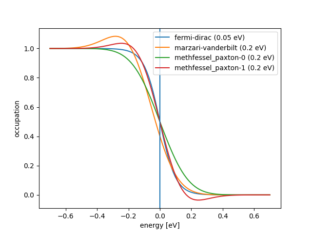
../_images/occupation_numbers.png — Occupation numbers for different distribution functions (value of `width` parameter in parenthesis)¶

For fixed occupations numbers use the gpaw.occupations.FixedOccupationNumbers class like this:

from gpaw.occupations import FixedOccupationNumbers
calc = GPAW(...,
            occupations=FixedOccupationNumbers([[1, 1, ..., 0, 0],
                                                [1, 1, ..., 0, 0]]))

Compensation charges¶

The compensation charges are expanded with correct multipoles up to and including $\ell=\ell_{max}$. Default value: lmax=2.

Charge¶

The default is charge neutral. The systems total charge may be set in units of the negative electron charge (i.e. charge=-1 means one electron more than the neutral).

Accuracy of the self-consistency cycle¶

The convergence keyword is used to set the convergence criteria for the SCF cycle. The default value is this dictionary:

{'energy': 0.0005,  # eV / electron
 'density': 1.0e-4,  # electrons / electron
 'eigenstates': 4.0e-8,  # eV^2 / electron
 'bands': 'occupied'}

In words:

The energy change (last 3 iterations) should be less than 0.5 meV per valence electron. (See Energy.)
The change in density (integrated absolute value of density change) should be less than 0.0001 electrons per valence electron. (See Density.)
The integrated value of the square of the residuals of the Kohn-Sham equations should be less than 4.0 $\times$ 10^-8 eV² per valence electron. This criterion does not affect LCAO calculations. (See Eigenstates.)
Only the bands that are occupied with electrons are converged.

If only a partial dictionary is provided, the remaining criteria will be set to their default values. E.g., convergence={'energy': 0.0001} will set the convergence criterion of energy to 0.1 meV and place all other criteria at their defaults.

Additional keywords, including 'forces', 'work function', and 'minimum iterations', can be set. You can also write your own criteria, and change other things about how the default criteria operate. See Custom convergence criteria for details on additional keywords and customization.

As the total energy and charge density depend only on the occupied states, unoccupied states do not contribute to the convergence criteria. However, with the 'bands' set to 'all', it is possible to force convergence also for the unoccupied states. One can also use {'bands': 200} to converge the lowest 200 bands. One can also write {'bands': -10} to converge all bands except the last 10. It is often hard to converge the last few bands in a calculation. Finally, one can also use {'bands': 'CBM+5.0'} to specify that bands up to the conduction band minimum plus 5.0 eV should be converged (for a metal, CBM is taken as the Fermi level).

Maximum number of SCF-iterations¶

The calculation will stop with an error if convergence is not reached in maxiter self-consistent iterations. You can also set a minimum number of iterations by employing a custom convergence criterion.

Where to send text output¶

The txt keyword defaults to the string '-', which means standard output. One can also give a file object (anything with a write method will do). If a string (different from '-') is passed to the txt keyword, a file with that name will be opened and used for output. Use txt=None to disable all text output.

Density mixing¶

Three parameters determine how GPAW does Pulay mixing of the densities:

beta: linear mixing coefficient
nmaxold: number of old densities to mix
weight: when measuring the change from input to output density, long wavelength changes are weighted weight times higher than short wavelength changes

For small molecules, the best choice is to use mixer=Mixer(beta=0.25, nmaxold=3, weight=1.0), which is what GPAW will choose if the system has zero-boundary conditions.

If your system is a big molecule or a cluster, it is an advantage to use something like mixer=Mixer(beta=0.05, nmaxold=5, weight=50.0), which is also what GPAW will choose if the system has periodic boundary conditions in one or more directions.

In spin-polarized calculations MixerDif will be used instead of Mixer.

See also the documentation on density mixing.

Fixed density calculation¶

When calculating band structures or when adding unoccupied states to calculation (and wanting to converge them) it is often useful to use existing density without updating it. This can be done using the gpaw.calculator.GPAW.fixed_density() method. This will use the density (e.g. one read from .gpw or existing from previous calculation) throughout the SCF-cycles (so called Harris calculation).

PAW datasets or pseudopotentials¶

The setups keyword is used to specify the name(s) of the setup files used in the calculation.

For a given element E, setup name NAME, and xc-functional ‘XC’, GPAW looks for the file E.NAME.XC or E.NAME.XC.gz (in that order) in the setup locations (see Installation of PAW datasets). Unless NAME='paw', in which case it will simply look for E.XC (or E.XC.gz). The setups keyword can be either a single string, or a dictionary.

If specified as a string, the given name is used for all atoms. If specified as a dictionary, each keys can be either a chemical symbol or an atom number. The values state the individual setup names.

The special key 'default' can be used to specify the default setup name. Thus setups={'default': 'paw'} is equivalent to setups='paw' which is the GPAW default.

As an example, the latest PAW setup of Na includes also the 6 semicore p states in the valence, in order to use non-default setup with only the 1 s electron in valence (Na.1.XC.gz) one can specify setups={'Na': '1'}

There exist three special names that, if used, do not specify a file name:

'ae' is used for specifying all-electron mode for an atom. I.e. no PAW or pseudo potential is used.
'sg15' specifies the SG15 optimized norm-conserving Vanderbilt pseudopotentials for the PBE functional. These have to be installed separately. Use gpaw install-data --sg15 {<dir>} to download and unpack the pseudopotentials into <dir>/sg15_oncv_upf_<version>. As of now, the SG15 pseudopotentials should still be considered experimental in GPAW. You can plot a UPF pseudopotential by running gpaw-upfplot <pseudopotential>. Here, <pseudopotential> can be either a direct path to a UPF file or the symbol or identifier to search for in the GPAW setup paths.
'hgh' is used to specify a norm-conserving Hartwigsen-Goedecker-Hutter pseudopotential (no installation necessary). Some elements have better semicore pseudopotentials. To use those, specify 'hgh.sc' for the elements or atoms in question.
'ghost' is used to indicated a ghost atom in LCAO mode, see Ghost atoms and basis set superposition errors.

If a dictionary contains both chemical element specifications and atomic number specifications, the latter is dominant.

An example:

setups={'default': 'soft', 'Li': 'hard', 5: 'ghost', 'H': 'ae'}

Indicates that the files named ‘hard’ should be used for lithium atoms, an all-electron potential is used for hydrogen atoms, atom number 5 is a ghost atom (even if it is a Li or H atom), and for all other atoms the files named ‘soft’ will be used.

Atomic basis set¶

The basis keyword can be used to specify the basis set which should be used in LCAO mode. This also affects the LCAO initialization in FD or PW mode, where initial wave functions are constructed by solving the Kohn-Sham equations in the LCAO basis.

If basis is a string, basis='basisname', then GPAW will look for files named symbol.basisname.basis in the setup locations (see Installation of PAW datasets), where symbol is taken as the chemical symbol from the Atoms object. If a non-default setup is used for an element, its name is included as symbol.setupname.basisname.basis.

If basis is a dictionary, its keys specify atoms or species while its values are corresponding basis names which work as above. Distinct basis sets can be specified for each atomic species by using the atomic symbol as a key, or for individual atoms by using an int as a key. In the latter case the integer corresponds to the index of that atom in the Atoms object. As an example, basis={'H': 'sz', 'C': 'dz', 7: 'dzp'} will use the sz basis for hydrogen atoms, the dz basis for carbon, and the dzp for whichever atom is number 7 in the Atoms object.

Note

If you want to use only the sz basis functinons from a dzp basis set, then you can use this syntax: basis='sz(dzp)'. This will read the basis functions for, say hydrogen, from the H.dzp.basis file. If the basis has a custom name, it is specified as 'szp(mybasis.dzp)'.

The value None (default) implies that the pseudo partial waves from the setup are used as a basis. This basis is always available; choosing anything else requires the existence of the corresponding basis set file in setup locations (see Installation of PAW datasets).

For details on the LCAO mode and generation of basis set files; see the LCAO documentation.

Eigensolver¶

The default solver for iterative diagonalization of the Kohn-Sham Hamiltonian is a simple Davidson method, (eigensolver='dav'), which seems to perform well in most cases. Sometimes more efficient/stable convergence can be obtained with a different eigensolver. One option is the RMM-DIIS (Residual minimization method - direct inversion in iterative subspace), (eigensolver='rmm-diis'), which performs well when only a few unoccupied states are calculated. Another option is the conjugate gradient method (eigensolver='cg'), which is stable but slower.

If parallellization over bands is necessary, then Davidson or RMM-DIIS must be used.

More control can be obtained by using directly the eigensolver objects:

from gpaw.eigensolvers import CG
calc = GPAW(..., eigensolver=CG(niter=5, rtol=0.20), ...)

Here, niter specifies the maximum number of conjugate gradient iterations for each band (within a single SCF step), and if the relative change in residual is less than rtol, the iteration for the band is not continued.

LCAO mode has its own eigensolvers. DirectLCAO eigensolver directly diagonalizes the Hamiltonian matrix instead of using an iterative method. One can also use Exponential Transformation Direct Minimization (ETDM) method (see Direct Minimization Methods) but it is not recommended to use it for metals because occupation numbers are not found variationally in ETDM.

Poisson solver¶

The poissonsolver keyword is used to specify a Poisson solver class or enable dipole correction.

The default Poisson solver in FD and LCAO mode is called FastPoissonSolver and uses a combination of Fourier and Fourier-sine transforms in combination with parallel array transposes. Meanwhile in PW mode, the Poisson equation is solved by dividing each planewave coefficient by the squared length of its corresponding wavevector.

The old default Poisson solver uses a multigrid Jacobian method. This example corresponds to the old default Poisson solver:

from gpaw import GPAW, PoissonSolver
calc = GPAW(...,
            poissonsolver=PoissonSolver(
                name='fd', nn=3, relax='J', eps=2e-10),
            ...)

The nn argument is the stencil, see Finite-difference stencils. The relax argument is the method, either 'J' (Jacobian) or 'GS' (Gauss-Seidel). The Gauss-Seidel method requires half as many iterations to solve the Poisson equation, but involves more communication. The Gauss-Seidel implementation also depends slightly on the domain decomposition used. The last argument, eps, is the convergence criterion.

Note

The Poisson solver is rarely a performance bottleneck, but it can sometimes perform poorly depending on the grid layout. This is mostly important in LCAO calculations, but can be good to know in general. See the LCAO notes on Poisson performance.

The poissonsolver keyword can also be used to specify that a dipole-layer correction should be applied along a given axis. The system should be non-periodic in that direction but periodic in the two other directions.

from gpaw import GPAW

correction = {'dipolelayer': 'xy'}
calc = GPAW(..., poissonsolver=correction, ...)

Without dipole correction, the potential will approach 0 at all non-periodic boundaries. With dipole correction, there will be a potential difference across the system depending on the size of the dipole moment.

Other parameters in this dictionary are forwarded to the Poisson solver:

GPAW(...,
     poissonsolver={'dipolelayer': 'xy', 'name': 'fd', 'relax': 'GS'},
     ...)

An alternative Poisson solver based on Fourier transforms is available for fully periodic calculations:

GPAW(..., poissonsolver={'name': 'fft'}, ...)

The FFT Poisson solver will reduce the dependence on the grid spacing and is in general less picky about the grid. It may be beneficial for non-periodic systems as well, but the system must be set up explicitly as periodic and hence should be well padded with vacuum in non-periodic directions to avoid unphysical interactions across the cell boundary.

Finite-difference stencils¶

GPAW can use finite-difference stencils for the Laplacian in the Kohn-Sham and Poisson equations. You can set the range of the stencil (number of neighbor grid points) used for the Poisson equation like this:

from gpaw import GPAW, PoissonSolver
calc = GPAW(..., poissonsolver=PoissonSolver(nn=n), ...)

This will give an accuracy of $O(h^{2n})$, where n must be between 1 and 6. The default value is n=3. Similarly, for the Kohn-Sham equation, you can use:

from gpaw import GPAW, FD
calc = GPAW(mode=FD(nn=n))

where the default value is also n=3.

In PW-mode, the interpolation of the density from the coarse grid to the fine grid is done with FFT’s. In FD and LCAO mode, tri-quintic interpolation is used (5. degree polynomium):

from gpaw import GPAW, FD
calc = GPAW(mode=FD(interpolation=n))
# or
from gpaw import GPAW, LCAO
calc = GPAW(mode=LCAO(interpolation=n))

The order of polynomium is $2n-1$, default value is n=3 and n must be between 1 and 4 (linear, cubic, quintic, heptic).

Using Hund’s rule for guessing initial magnetic moments¶

With hund=True, the calculation will become spinpolarized, and the initial ocupations, and magnetic moments of all atoms will be set to the values required by Hund’s rule. You may further wish to specify that the total magnetic moment be fixed, by passing e.g. occupations={'name': ..., 'fixmagmom': True}. Any user specified magnetic moment is ignored. Default is False.

External potential¶

Example:

from gpaw.external import ConstantElectricField
calc = GPAW(..., external=ConstantElectricField(2.0, [1, 0, 0]), ...)

Output verbosity¶

By default, only a limited number of information is printed out for each SCF step. It is possible to obtain more information (e.g. for investigating convergen problems in more detail) by verbose=1 keyword.

Communicator object¶

By specifying a communicator object, it is possible to use only a subset of processes for the calculator when calculating e.g. different atomic images in parallel. See Running different calculations in parallel for more details.

Total Energies¶

The GPAW code calculates energies relative to the energy of separated reference atoms, where each atom is in a spin-paired, neutral, and spherically symmetric state - the state that was used to generate the setup. For a calculation of a molecule, the energy will be minus the atomization energy and for a solid, the resulting energy is minus the cohesive energy. So, if you ever get positive energies from your calculations, your system is in an unstable state!

Note

You don’t get the true atomization/cohesive energy. The true number is always lower, because most atoms have a spin-polarized and non-spherical symmetric ground state, with an energy that is lower than that of the spin-paired, and spherically symmetric reference atom.

Restarting a calculation¶

The state of a calculation can be saved to a file like this:

>>> calc.write('H2.gpw')

The file H2.gpw is a binary file containing wave functions, densities, positions and everything else (also the parameters characterizing the PAW calculator used for the calculation).

If you want to restart the $\rm{H}_2$ calculation in another Python session at a later time, this can be done as follows:

>>> from gpaw import *
>>> atoms, calc = restart('H2.gpw')
>>> print(atoms.get_potential_energy())

Everything will be just as before we wrote the H2.gpw file. Often, one wants to restart the calculation with one or two parameters changed slightly. This is simple to do. Suppose you want to change the number of grid points:

>>> atoms, calc = restart('H2.gpw', gpts=(20, 20, 20))
>>> print(atoms.get_potential_energy())

Tip

There is an alternative way to do this, that can be handy sometimes:

>>> atoms, calc = restart('H2.gpw')
>>> calc.set(gpts=(20, 20, 20))
>>> print(atoms.get_potential_energy())

More details can be found on the Restart files page.

Customizing behaviour through observers¶

An observer function can be attached to the calculator so that it will be executed every N iterations during a calculation. The below example saves a differently named restart file every 5 iterations:

calc = GPAW(...)

occasionally = 5

class OccasionalWriter:
    def __init__(self):
        self.iter = 0

    def write(self):
        calc.write('filename.%03d.gpw' % self.iter)
        self.iter += occasionally

calc.attach(OccasionalWriter().write, occasionally)

Command-line options¶

I order to run GPAW in debug-mode, e.g. check consistency of arrays passed to C-extensions, use Python’s -d option:

$ python3 -d script.py

If you run Python through the gpaw python command, then you can run your script in dry-run mode like this:

$ gpaw python --dry-run=N script.py

This will print out the computational parameters and estimate memory usage, and not perform an actual calculation. Parallelization settings that would be employed when run on N cores will also be printed.

Tip

If you need extra parameters from the command-line for development work:

$ python3 -X a=1 -X b
>>> import sys
>>> sys._xoptions
{'a': '1', 'b': True}