Bethe-Salpeter Equation - Theory

Introduction

The BSE object calculates optical and dielectric properties of extended systems including the electron-hole interaction (excitonic effects).

The four point Bethe-Salpeter equation

Please refer to Linear dielectric response of an extended system: theory for the documentation on the density response function \(\chi\). Most of the derivations in this page follow reference [1].

The following diagrams [1] representing the four point Bethe-Salpeter equation:

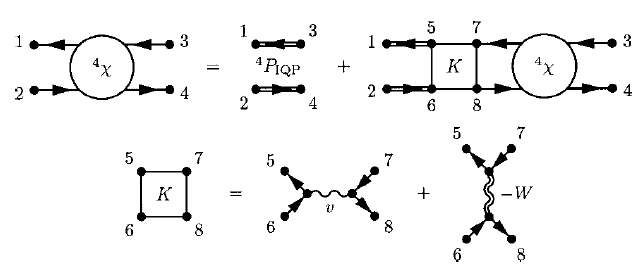
It can be written as:

(1)\[\begin{split}&\chi(\mathbf{r}_1, \mathbf{r}_2, \mathbf{r}_3, \mathbf{r}_4; \omega) = \chi^{0}(\mathbf{r}_1, \mathbf{r}_2, \mathbf{r}_3, \mathbf{r}_4; \omega) \\ & + \int d \mathbf{r}_5 d \mathbf{r}_6 d \mathbf{r}_7 d \mathbf{r}_8 \chi^{0}(\mathbf{r}_1, \mathbf{r}_2, \mathbf{r}_5, \mathbf{r}_6; \omega) K( \mathbf{r}_5, \mathbf{r}_6, \mathbf{r}_7, \mathbf{r}_8; \omega) \chi(\mathbf{r}_7, \mathbf{r}_8, \mathbf{r}_3, \mathbf{r}_4; \omega)\end{split}\]

where

\[K = V - W = \frac{1}{| \mathbf{r}_5 - \mathbf{r}_7|} \delta_{ \mathbf{r}_5, \mathbf{r}_6} \delta_{ \mathbf{r}_7, \mathbf{r}_8} - \int d \mathbf{r} \frac{\epsilon^{-1}( \mathbf{r}_5, \mathbf{r}; \omega )} {| \mathbf{r} - \mathbf{r}_6|} \delta_{ \mathbf{r}_5, \mathbf{r}_7} \delta_{ \mathbf{r}_6, \mathbf{r}_8}\]

The density response function \(\chi\), defined as \(\chi(\mathrm{r}, \mathrm{r}^{\prime}) = \delta n(\mathrm{r}) / \delta V_{ext}(\mathrm{r}^{\prime})\), has a form of

(2)\[\chi(\mathbf{r}_1, \mathbf{r}_2, \mathbf{r}_3, \mathbf{r}_4; \omega) = \chi(\mathbf{r}_1, \mathbf{r}_3; \omega) \delta_{ \mathbf{r}_1, \mathbf{r}_2} \delta_{ \mathbf{r}_3, \mathbf{r}_4}\]

The above equation also applies for the non interacting density response function \(\chi^0\). As a result, the four point Bethe-Salpeter equation (1) can be reduced to:

(3)\[\begin{split}\chi(\mathbf{r}, \mathbf{r}^{\prime}; \omega) &= \chi^0(\mathbf{r}, \mathbf{r}^{\prime}; \omega) + \int d \mathbf{r}_5 d \mathbf{r}_7 \chi^0(\mathbf{r}, \mathbf{r}_5; \omega) \frac{1}{| \mathbf{r}_5 - \mathbf{r}_7|} \chi(\mathbf{r}_7, \mathbf{r}^{\prime}; \omega) \\ &+ \int d \mathbf{r}_5 d \mathbf{r}_6 d \mathbf{r}^{\prime \prime} \chi^0(\mathbf{r},\mathbf{r}, \mathbf{r}_5, \mathbf{r}_6; \omega) \frac{\epsilon^{-1}( \mathbf{r}_5, \mathbf{r}^{\prime \prime}; \omega )} {| \mathbf{r}^{\prime \prime} - \mathbf{r}_6|} \chi(\mathbf{r}_5, \mathbf{r}_6, \mathbf{r}^{\prime}, \mathbf{r}^{\prime}; \omega)\end{split}\]

Transform using electron-hole pair basis

Since for each excitation, only a limited number of electron-hole pairs will contribute , the above equation can be effectively transformed to electron-hole pair space. Supposed that the eigenfunctions \(\psi_{n}\) of the effective Kohn-Sham hamiltonian form an orthonormal and complete basis set, any four point function \(S\) can then be transformed as

(4)\[\begin{split}S(\mathbf{r}_1, \mathbf{r}_2, \mathbf{r}_3, \mathbf{r}_4; \omega) = \sum_{n_1 n_2 n_3 n_4} \psi^{\ast}_{n_{1}}(\mathbf{r}_1) \psi_{n_{2}}(\mathbf{r}_2) \psi_{n_{3}}(\mathbf{r}_3) \psi^{\ast}_{n_{4}}(\mathbf{r}_4) S_{\begin{array}{l} n_1 n_2 \\ n_3 n_4 \end{array}} (\omega)\end{split}\]

The non interacting density response function \(\chi^0\)

(5)\[ \chi^0(\mathbf{r}_1, \mathbf{r}_2, \mathbf{r}_3, \mathbf{r}_4; \omega) = \sum_{n n^{\prime}} \frac{f_n - f_{n^{\prime}}}{\epsilon_n - \epsilon_{n^{\prime}}-\omega} \psi^{\ast}_n(\mathbf{r}_1) \psi_{n^{\prime}}(\mathbf{r}_2) \psi_n(\mathbf{r}_3) \psi^{\ast}_{n^{\prime}}(\mathbf{r}_4)\]

is then diagonal in the electron-hole basis with

(6)\[\begin{split} \chi^0_{\begin{array}{l} n_1 n_2 \\ n_3 n_4 \end{array}} (\omega) = \frac{f_{n_2} - f_{n_1}}{\epsilon_{n_2} - \epsilon_{n_1}-\omega} \delta_{n_1, n_3} \delta_{n_2, n_4}\end{split}\]

Substitute Eq. (4) and (5) into Eq. (3) and by using Eq. (2) ,the four point Bethe-Salpeter equation in electron-hole pair space becomes

(7)\[\begin{split} \chi_{\begin{array}{l} n_1 n_2 \\ n_3 n_4 \end{array}} (\omega) = \chi^0_{n_1 n_2} (\omega) \left[ \delta_{n_1 n_3} \delta_{n_2 n_4} + \sum_{n_5 n_6} K_{\begin{array}{l} n_1 n_2 \\ n_5 n_6 \end{array}} (\omega) \chi_{\begin{array}{l} n_5 n_6 \\ n_3 n_4 \end{array}} (\omega) \right]\end{split}\]

with \(K = V - W\) and

(8)\[\begin{split} V_{\begin{array}{l} n_1 n_2 \\ n_5 n_6 \end{array}} = \int d \mathbf{r} d \mathbf{r}^{\prime} \psi_{n_1}(\mathbf{r}) \psi_{n_2}^{\ast}(\mathbf{r}) \frac{1}{| \mathbf{r}-\mathbf{r}^{\prime} |} \psi^{\ast}_{n_5}(\mathbf{r}^{\prime}) \psi_{n_6}(\mathbf{r}^{\prime})\end{split}\]

(9)\[\begin{split} W_{\begin{array}{l} n_1 n_2 \\ n_5 n_6 \end{array}} (\omega) = \int d \mathbf{r} d \mathbf{r}^{\prime} d \mathbf{r}^{\prime \prime} \psi_{n_1}(\mathbf{r}) \psi_{n_2}^{\ast}(\mathbf{r}^{\prime}) \frac{\epsilon^{-1}( \mathbf{r}, \mathbf{r}^{\prime \prime}; \omega )}{| \mathbf{r}^{\prime \prime}-\mathbf{r}^{\prime} |} \psi^{\ast}_{n_5}(\mathbf{r}) \psi_{n_6}(\mathbf{r}^{\prime})\end{split}\]

Bethe-Salpeter equation as an effective two-particle Hamiltonian

In order to solve Eq. (7), one has to invert a matrix for each frequency. This problem can be reformulated as an effective eigenvalue problem. Rewrite Eq. (7) as

\[\begin{split}\sum_{n_5 n_6} \left[ \delta_{n_1 n_5} \delta_{n_2 n_6} - \chi^0_{n_1 n_2}(\omega) K_{\begin{array}{l} n_1 n_2 \\ n_5 n_6 \end{array}} (\omega) \right] \chi_{\begin{array}{l} n_5 n_6 \\ n_3 n_4 \end{array}} (\omega) = \chi^0_{n_1 n_2}(\omega)\end{split}\]

Insert Eq. (6) into the above equation, one gets

(10)\[\begin{split}\sum_{n_5 n_6} \left[ (\epsilon_{n_2} - \epsilon_{n_1}-\omega) \delta_{n_1 n_5} \delta_{n_2 n_6} - (f_{n_2} - f_{n_1}) K_{\begin{array}{l} n_1 n_2 \\ n_5 n_6 \end{array}} (\omega) \right] \chi_{\begin{array}{l} n_5 n_6 \\ n_3 n_4 \end{array}} (\omega) = f_{n_2} - f_{n_1}\end{split}\]

By using a static interaction kernel \(K(\omega=0)\), an effective frequency-indendepnt two particle Hamiltonian is defined as:

(11)\[\begin{split}\mathcal{H}_{\begin{array}{l} n_1 n_2 \\ n_5 n_6 \end{array}} \equiv (\epsilon_{n_2} - \epsilon_{n_1}) \delta_{n_1 n_5} \delta_{n_2 n_6} - (f_{n_2} - f_{n_1}) K_{\begin{array}{l} n_1 n_2 \\ n_5 n_6 \end{array}}\end{split}\]

Inserting the above effective Hamiltonian into Eq. (10), one can then write

(12)\[\begin{split}\chi_{\begin{array}{l} n_1 n_2 \\ n_3 n_4 \end{array}} = \left[ \mathcal{H} - I \omega \right]^{-1}_{\begin{array}{l} n_1 n_2 \\ n_3 n_4 \end{array}} (f_{n_2} - f_{n_1})\end{split}\]

where \(I\) is an identity matrix that has the same size as \(\mathcal{H}\).

In the following subsection, we will show that by diagonalizing the Hamiltonian matrix \(\mathcal{H}\), the obtained eigenvalues are the excitations energies of elementary electronic excitations such as excitons or plasmons, while the eigenvectors are related to the strength of the electronic excitations.

The spectral representation of the inverse two-particle Hamiltonian is

(13)\[\begin{split}\left[ \mathcal{H} - I \omega \right]^{-1}_{\begin{array}{l} n_1 n_2 \\ n_3 n_4 \end{array}} = \sum_{\lambda \lambda^{\prime}} \frac{A^{n_1 n_2}_{\lambda} A^{n_3 n_4}_{\lambda^{\prime}} N^{-1}_{\lambda \lambda^{\prime}}}{E_{\lambda} - \omega}\end{split}\]

with the eigenvalues \(E_{\lambda}\) and eigenvectors \(A_{\lambda}\) given by

\[\mathcal{H} A_{\lambda} = E_{\lambda} A_{\lambda}\]

and the overlap matrix \(N_{\lambda \lambda^{\prime} }\) defined by

\[N_{\lambda \lambda^{\prime}} \equiv \sum_{n_1 n_2} [A_{\lambda}^{n_1 n_2}]^{\ast} A_{\lambda^{\prime}}^{n_1 n_2}\]

If the Hamiltonian \(\mathcal{H}\) is Hermitian, the eigenvectors \(A_{\lambda}\) are then orthogonal and

\[N_{\lambda \lambda^{\prime}} = \delta_{\lambda \lambda^{\prime}}\]

Explicit kpoint dependence

In this subsection, the kpoint dependence of the eigenstates is written explicitly.

The effective two particle Hamiltonian in Eq. (11) becomes

\[\begin{split}\mathcal{H}_{\begin{array}{l} n_1 n_2 \mathbf{k}_1 \\ n_5 n_6 \mathbf{k}_5 \end{array}} ( \mathbf{q}) \equiv (\epsilon_{n_2 \mathbf{k}_1 + \mathbf{q}} - \epsilon_{n_1 \mathbf{k}_1}) \delta_{n_1 n_5} \delta_{n_2 n_6} \delta_{\mathbf{k}_1 \mathbf{k}_5} - (f_{n_2 \mathbf{k}_1 + \mathbf{q}} - f_{n_1 \mathbf{k}_1}) K_{\begin{array}{l} n_1 n_2 \mathbf{k}_1 \\ n_5 n_6 \mathbf{k}_5 \end{array}} ( \mathbf{q})\end{split}\]

where \(K=V-W\) and according to Eq. (8) and (9),

(14)\[\begin{split} V_{\begin{array}{l} n_1 n_2 \mathbf{k}_1 \\ n_5 n_6 \mathbf{k}_5 \end{array}} ( \mathbf{q}) = \int d \mathbf{r} d \mathbf{r}^{\prime} \psi_{n_1 \mathbf{k}_1}(\mathbf{r}) \psi_{n_2 \mathbf{k}_1 + \mathbf{q}}^{\ast}(\mathbf{r}) \frac{1}{| \mathbf{r}-\mathbf{r}^{\prime} |} \psi^{\ast}_{n_5 \mathbf{k}_5}(\mathbf{r}^{\prime}) \psi_{n_6 \mathbf{k}_5 + \mathbf{q}}(\mathbf{r}^{\prime})\end{split}\]

(15)\[\begin{split} W_{\begin{array}{l} n_1 n_2 \mathbf{k}_1 \\ n_5 n_6 \mathbf{k}_5 \end{array}} ( \mathbf{q}) = \int d \mathbf{r} d \mathbf{r}^{\prime} \psi_{n_1 \mathbf{k}_1}(\mathbf{r}) \psi_{n_2 \mathbf{k}_1 + \mathbf{q}}^{\ast}(\mathbf{r}^{\prime}) \frac{\epsilon^{-1}( \mathbf{r}, \mathbf{r}^{\prime}; \omega=0 )}{| \mathbf{r}-\mathbf{r}^{\prime} |} \psi^{\ast}_{n_5 \mathbf{k}_5}(\mathbf{r}) \psi_{n_6 \mathbf{k}_5 + \mathbf{q}}(\mathbf{r}^{\prime})\end{split}\]

The response function in the electron-hole pair space, according to Eq. (12) and (13) becomes

(16)\[\begin{split}\chi_{\begin{array}{l} n_1 n_2 \mathbf{k}_1 \\ n_3 n_4 \mathbf{k}_3 \end{array}} (\mathbf{q}, \omega) = \sum_{\lambda \lambda^{\prime}} \frac{A^{n_1 n_2 \mathbf{k}_1}_{\lambda} A^{n_3 n_4 \mathbf{k}_3}_{\lambda^{\prime}} N^{-1}_{\lambda \lambda^{\prime}}}{E_{\lambda} - \omega} (f_{n_2 \mathbf{k}_1 + \mathbf{q}} - f_{n_1 \mathbf{k}_1})\end{split}\]

Transform between electron-hole pair space and reciprocal space

The physical quantities such as macroscopic dielectric function (refer to Dielectric function and its relation to spectra) are related to the long wavelength limit \((\mathbf{G}=0, \mathbf{G}^{\prime}=0)\) component of the response function \(\chi_{\mathbf{G} \mathbf{G}^{\prime}}\). Its relation to the response function in electron-hole pair space \(\chi_{\begin{array}{l} n_1 n_2 \mathbf{k}_1\\ n_3 n_4 \mathbf{k}_3 \end{array}}\) is written as

(17)\[\begin{split}\chi_{\mathbf{G} \mathbf{G}^{\prime}} (\mathbf{q}, \omega) = \frac{1}{\Omega} \sum_{\begin{array}{l} n_1 n_2 \mathbf{k}_1 \\ n_3 n_4 \mathbf{k}_3 \end{array}} \chi_{\begin{array}{l} n_1 n_2 \mathbf{k}_1\\ n_3 n_4 \mathbf{k}_3 \end{array}} (\mathbf{q},\omega) \ \ \rho_{\begin{array}{l} n_1 \mathbf{k}_1 \\ n_2 \mathbf{k}_1 + \mathbf{q} \end{array}} (\mathbf{G}) \ \ \rho^{\ast}_{\begin{array}{l} n_3 \mathbf{k}_3 \\ n_4 \mathbf{k}_3 + \mathbf{q} \end{array}} (\mathbf{G}^{\prime})\end{split}\]

where the charge density matrix \(\rho (\mathbf{G})\) is defined as:

\[\begin{split}\rho_{\begin{array}{l} n_1 \mathbf{k}_1 \\ n_2 \mathbf{k}_1 + \mathbf{q} \end{array}} (\mathbf{G}) \equiv \langle \psi_{n_1 \mathbf{k}_1} | e^{-i(\mathbf{q}+\mathbf{G}) \cdot \mathbf{r} } | \psi_{n_2 \mathbf{k}_1 + \mathbf{q}} \rangle\end{split}\]

Employing Fourier transform

\[\frac{1}{| \mathbf{r}-\mathbf{r}^{\prime} |} = \frac{1}{\Omega} \sum_{\mathbf{q} \mathbf{G}} \frac{4\pi}{ | \mathbf{q} + \mathbf{G}|^2 } e^{i ( \mathbf{q} + \mathbf{G}) \cdot ( \mathbf{r} - \mathbf{r}^{\prime} ) }\]

\[\int d \mathbf{r}^{\prime \prime}\frac{\epsilon^{-1}(\mathbf{r},\mathbf{r}^{\prime \prime}) }{| \mathbf{r}^{\prime \prime}-\mathbf{r}^{\prime} |} = \frac{1}{\Omega} \sum_{\mathbf{q} \mathbf{G} \mathbf{G}^{\prime} } e^{i ( \mathbf{q} + \mathbf{G}) \cdot \mathbf{r} } \frac{4\pi \epsilon^{-1}_{\mathbf{G} \mathbf{G}^{\prime}} (\mathbf{q}) }{ | \mathbf{q} + \mathbf{G}^{\prime}|^2 } e^{-i ( \mathbf{q} + \mathbf{G}^{\prime}) \cdot \mathbf{r}^{\prime} }\]

where \(\Omega\) is the volume of the unit cell, \(V\) and \(W\) in Eq. (14) and (15) can then be written respectively as

(18)\[\begin{split}V_{\begin{array}{l} n_1 n_2 \mathbf{k}_1 \\ n_5 n_6 \mathbf{k}_5 \end{array}} ( \mathbf{q}) =\sum_{\mathbf{G}} \rho^{\ast}_{\begin{array}{l} n_1 \mathbf{k}_1 \\ n_2 \mathbf{k}_1 + \mathbf{q} \end{array}} (\mathbf{G}) \ \frac{4\pi}{| \mathbf{q} + \mathbf{G}|^2} \ \rho_{\begin{array}{l} n_5 \mathbf{k}_5 \\ n_6 \mathbf{k}_5 + \mathbf{q} \end{array}} (\mathbf{G})\end{split}\]

\[\begin{split}W_{\begin{array}{l} n_1 n_2 \mathbf{k}_1 \\ n_5 n_6 \mathbf{k}_5 \end{array}} ( \mathbf{q}) = \sum_{\mathbf{G} \mathbf{G}^{\prime}} \rho^{\ast}_{\begin{array}{l} n_1 \mathbf{k}_1 \\ n_5 \mathbf{k}_5 \end{array}} (\mathbf{G}) \ \frac{4\pi \epsilon^{-1}_{\mathbf{G} \mathbf{G}^{\prime}} (\mathbf{k}_5-\mathbf{k}_1; \omega=0) }{| \mathbf{k}_5-\mathbf{k}_1 + \mathbf{G}|^2} \ \rho_{\begin{array}{l} n_2 \mathbf{k}_1 + \mathbf{q} \\ n_6 \mathbf{k}_5 + \mathbf{q} \end{array}} (\mathbf{G}^{\prime})\end{split}\]

Dielectric function and its relation to spectra

The dielectric matrix is related to the density response matrix by

\[\epsilon^{-1}_{\mathbf G \mathbf G^{\prime}}(\mathbf q, \omega) = \delta_{\mathbf G \mathbf G^{\prime}} + \frac{4\pi}{|\mathbf q + \mathbf G|^2} \chi_{\mathbf G \mathbf G^{\prime}}(\mathbf q, \omega)\]

Electron energy loss spectra (EELS) is propotional to \(-\mathrm{Im} \epsilon^{-1}_{00}\):

\[\mathrm{EELS} \propto -\mathrm{Im} \epsilon^{-1}_{00}(\mathbf q, \omega) = - \frac{4\pi}{|\mathbf{q}|^2} \mathrm{Im} \chi_{00}(\mathbf q, \omega)\]

As shown in Dielectric function and its relation to spectra, optical absorption spectra (ABS) is \(\mathrm{Im} \epsilon_M\). Instead of calculating from \(\epsilon^{-1}_{00}\), \(\epsilon_M\) can also be constructed from a modified response function \(\bar{\chi}\) by

\[\epsilon_M (\omega) = 1 - \frac{4\pi}{|\mathbf{q}|^2} \bar{\chi}_{00}(\mathbf{q}\rightarrow 0, \omega)\]

\[\mathrm{ABS} = \mathrm{Im} \epsilon_M (\omega) = -\frac{4\pi}{|\mathbf{q}|^2} \mathrm{Im}\bar{\chi}_{00}(\mathbf{q}\rightarrow 0, \omega)\]

The modified response function \(\bar{\chi}\) is constructed in the same way as \(\chi\), except that the long range Coulomb interaction for kernel \(V\) in Eq. (18) is excluded so that

\[\begin{split} \bar{V}_{\begin{array}{l} n_1 n_2 \mathbf{k}_1 \\ n_5 n_6 \mathbf{k}_5 \end{array}} ( \mathbf{q}) =\sum_{\mathbf{G} \neq 0} \rho^{\ast}_{\begin{array}{l} n_1 \mathbf{k}_1 \\ n_2 \mathbf{k}_1 + \mathbf{q} \end{array}} (\mathbf{G}) \ \frac{4\pi}{| \mathbf{q} + \mathbf{G}|^2} \ \rho_{\begin{array}{l} n_5 \mathbf{k}_5 \\ n_6 \mathbf{k}_5 + \mathbf{q} \end{array}} (\mathbf{G})\end{split}\]

The implementation flowchart

Here is a short summary for the actual implementation:

1. Construct the effective two particle Hamiltonian (using notation \(S \equiv \left\{ n_1 n_2 \mathbf{k}_1; \mathbf{q} \right\}\) and \(S^{\prime} \equiv \left\{ n_3 n_4 \mathbf{k}_3; \mathbf{q} \right\}\))

\[\mathcal{H}_{SS^{\prime}} (\mathbf{q}) = \epsilon_S \delta_{SS^{\prime}} - f_S K_{SS^{\prime}} ( \mathbf{q})\]

where

(19)\[\epsilon_S = \epsilon_{n_2 \mathbf{k}_1 + \mathbf{q}} - \epsilon_{n_1 \mathbf{k}_1}\]

\[f_S = f_{n_2 \mathbf{k}_1 + \mathbf{q}} - f_{n_1 \mathbf{k}_1}\]

with \(K=V-0.5W\), where 0.5 accounts for the fact that only singlet excitations are allowed in the optical absorption and \(W\) are diagonal in spin. The Coulomb interaction \(V\) is given by

\[V_{SS^{\prime}} (\mathbf{q}) = \sum_{\mathbf{G} \neq 0} \rho^{\ast}_S(\mathbf{G}) \frac{4\pi}{| \mathbf{q} + \mathbf{G}|^2} \rho_{S^{\prime}}(\mathbf{G}) \ \ (\mathrm{ABS})\]

\[V_{SS^{\prime}} (\mathbf{q}) = \sum_{\mathbf{G}} \rho^{\ast}_S(\mathbf{G}) \frac{4\pi}{| \mathbf{q} + \mathbf{G}|^2} \rho_{S^{\prime}}(\mathbf{G}) \ \ (\mathrm{EELS})\]

where

\[\rho_{S}(\mathbf{G}) = \langle \psi_{n_1 \mathbf{k}_1} | e^{-i(\mathbf{q}+\mathbf{G}) \cdot \mathbf{r} } | \psi_{n_2 \mathbf{k}_1 + \mathbf{q}} \rangle\]

The screened interaction kernel \(W\) is given by

\[\begin{split}W_{SS^{\prime}} ( \mathbf{q}) = \sum_{\mathbf{G} \mathbf{G}^{\prime}} \rho^{\ast}_{\begin{array}{l} n_1 \mathbf{k}_1 \\ n_3 \mathbf{k}_3 \end{array}} (\mathbf{G}) \ \frac{4\pi \epsilon^{-1}_{\mathbf{G} \mathbf{G}^{\prime}} (\mathbf{k}_3 - \mathbf{k}_1; \omega=0) }{| \mathbf{k}_3 - \mathbf{k}_1 + \mathbf{G}|^2} \ \rho_{\begin{array}{l} n_2 \mathbf{k}_1 + \mathbf{q} \\ n_4 \mathbf{k}_3 + \mathbf{q} \end{array}} (\mathbf{G}^{\prime})\end{split}\]

2. Diagonalize \(\mathcal{H}_{SS^{\prime}}\) with the eigenvalues \(E_{\lambda}\) and eigenvectors \(A_{\lambda}\) given by

\[\mathcal{H} A_{\lambda} = E_{\lambda} A_{\lambda}\]

and the overlap matrix \(N_{\lambda \lambda^{\prime} }\) defined by

\[N_{\lambda \lambda^{\prime}} \equiv \sum_{S} [A_{\lambda}^{S}]^{\ast} A_{\lambda^{\prime}}^{S}\]

The eigenvalues \(E_{\lambda}\), which correpond to the poles of \(\chi\), give the excitation energies of the elementary electron excitations.

3. The spectra (both EELS and ABS) are calculated by

\[-\frac{4\pi}{|\mathbf{q}|^2} \mathrm{Im} \chi_{00}(\mathbf q, \omega) = - \frac{4\pi}{|\mathbf{q}|^2 \Omega} \sum_{\lambda \lambda^{\prime}} \sum_{SS^{\prime}} \frac{ f_S A^{S}_{\lambda} A^{S^{\prime}}_{\lambda^{\prime}} N^{-1}_{\lambda \lambda^{\prime}}}{E_{\lambda} - \omega} \ \rho_S(0) \rho_{S^{\prime}}(0)\]

Tamm-Dancoff approximation

The Tamm-Dancoff approximation corresponds to \(\epsilon_S >= 0\) in Eq. (19).

[1] (1,2)

G. Onida, L. Reining and A. Rubio, Electronic excitations: density-functional versus many-body Green’s-function approaches, Rev. Mod. Phys. 74, 601 (2002)