Electronic Band Structure Unfolding for Supercell Calculations
Brief theory overview
Due to the many electrons in the unit cell, the electronic band structure of a supercell (SC) calculation is in general quite messy. However, supercell calculations are usually performed in order to allow for minor modification of the crystal structure, i.e. defects, distortions etc. In this cases it could be useful to investigate, up to what extent, the electronic structure of the non-defective is preserved. To this scope, unfolding the band structure of the SC to the one of the primitive cell (PC) becomes handy.
Consider the case where the basis vectors of the SC and PC satisfy:
\[\underline{\vec{A}} = \underline{M}\cdot\underline{\vec{a}},\]
where \(\underline{\vec{A}}\) and \(\underline{\vec{a}}\) are matrices with the cell basis vectors as rows and \(\underline{M}\) the trasformation matrix. As a general convention, capital and lower caseletters indicate quantities in the SC and PC respectively. A similar relation holds in reciprocal space:
\[\underline{\vec{B}} = \underline{M}^{-1}\cdot\underline{\vec{b}},\]
with obvious notation. Now given a \(\vec{k}\) in the PBZ there is only a \(\vec{K}\) in the SBZ to which it folds into, and the two vectors are related by a reciprocal lattice vector \(\vec{G}\) in the SBZ:
\[\vec{k} = \vec{K}+\vec{G},\]
whereas the opposite is not true since a \(\vec{K}\) unfolds into a subset of PBZ vectors \(\left\{\vec{k}_i\right\}\).
We are in general interested in finding the spectral function of the PC calculation starting from eigenvalues and eigenfunctions of the SC one. Such a spectral function can be calculated as follows:
\[A(\vec{k},\epsilon) = \sum_m P_{\vec{K}m}(\vec{k}) \delta(\epsilon_{\vec{K}m}-\epsilon).\]
Remember that \(\vec{k}\) and \(\vec{K}\) are related to each other and this is why we made \(\vec{K}\) appear on the RHS. In the previous equation, \(P_{\vec{K}m}(\vec{k})\) are the weights defined by:
\[P_{\vec{K}m}(\vec{k}) = \sum_n |\langle\vec{K}m|\vec{k}n\rangle|^2\]
which give information about how much of the character \(|\vec{k}n\rangle\) is preserved in \(|\vec{K}n\rangle\). From the expression above, it seems that calculating the weights requires the knowledge of the PC eigenstates. However, V.Popescu and A.Zunger show in [1] that weights can be found using only SC quantities, according to:
\[P_{\vec{K}m}(\vec{k}) = \sum_{sub\{\vec{G}\}} |C_{\vec{K}m}(\vec{G}+\vec{k}-\vec{K})|^2\]
where \(C_{\vec{K}m}\) are the Fourier coefficients of the eigenstate \(|\vec{K}m\rangle\) and \(sub\{\vec{G}\}\) a subset of reciprocal space vectors of the SC, specifically the ones that match the reciprocal space vectors of the PC. This is the method implemented in GPAW and it works in ‘realspace’, ‘lcao’ and ‘pw’ with or without spin-orbit.
Band Structure Unfolding for MoS2 supercell with single sulfur vacancy
Groundstate calculation
First, we need a regular groundstate calculation for a \(3\times3\) supercell with a sulfur vacancy. For supercell calculation it is convenient to use ‘lcao’ with a ‘dzp’ basis.
from ase.build import mx2
from gpaw import GPAW, FermiDirac

structure = mx2(formula='MoS2', kind='2H', a=3.184, thickness=3.127,
                size=(3, 3, 1), vacuum=7.5)
structure.pbc = (1, 1, 1)

# Create vacancy
del structure[2]

calc = GPAW(mode='lcao',
            basis='dzp',
            xc='LDA',
            kpts=(4, 4, 1),
            occupations=FermiDirac(0.01),
            txt='gs_3x3_defect.txt')

structure.calc = calc
structure.get_potential_energy()
calc.write('gs_3x3_defect.gpw', 'all')
It takes a few minutes if run in parallel. The last line in the script creates a .gpw file which contains all the informations of the system, including the wavefunctions.
Band path in the PBZ and finding the corresponding \(\vec{K}\) in the SBZ
Next, we set up the path in the PBZ along which we want to calculate the spectral function, we define the transformation matrix M, and find the corresponding \(\vec{K}\) in the SBZ.
from ase.build import mx2

from gpaw import GPAW
from gpaw.unfold import Unfold, find_K_from_k

a = 3.184
PC = mx2(a=a).get_cell(complete=True)
bp = PC.get_bravais_lattice().bandpath('MKG', npoints=48)
x, X, _ = bp.get_linear_kpoint_axis()

M = [[3, 0, 0], [0, 3, 0], [0, 0, 1]]

Kpts = []
for k in bp.kpts:
    K = find_K_from_k(k, M)[0]
    Kpts.append(K)
Non self-consistent calculation at the \(\vec{K}\) points
Once we have the relevant \(\vec{K}\) we have to calculate eigenvalues and eigenvectors; we can do that non self-consistently.
calc_bands = GPAW('gs_3x3_defect.gpw').fixed_density(
    kpts=Kpts,
    symmetry='off',
    nbands=220,
    convergence={'bands': 200})

calc_bands.write('bands_3x3_defect.gpw', 'all')
Unfolding the bands and calculating Spectral Function
We are now ready to proceed with the unfolding. First we set up the
Unfold object.
unfold = Unfold(name='3x3_defect',
                calc='bands_3x3_defect.gpw',
                M=M,
                spinorbit=False)
and then we call the function for calculating the spectral function.
unfold.spectral_function(kpts=bp.kpts, x=x, X=X,
                         points_name=['M', 'K', 'G'])
This can be run in parallel over kpoints, and you may want to do that since the supercell is relatively big.
Note
The function produces two outputs, ‘weights_3x3_defects.pckl’ containing the eigenvalues \(\epsilon_{\vec{K}m}\) and the weights \(P_{\vec{K}m}(\vec{k})\) and ‘sf_3x3_defects.pckl’ which contains the spectral function and the corresponding energy array.
Plotting Spectral Function
Finally you can plot the spectral function using an utility function included
in gpaw.unfold module.
# web-page: sf_3x3_defect.png
from gpaw import GPAW
from gpaw.unfold import plot_spectral_function

calc = GPAW('gs_3x3_defect.gpw', txt=None)
ef = calc.get_fermi_level()

plot_spectral_function(filename='sf_3x3_defect',
                       color='blue',
                       eref=ef,
                       emin=-3,
                       emax=3)
which will produce the following image:
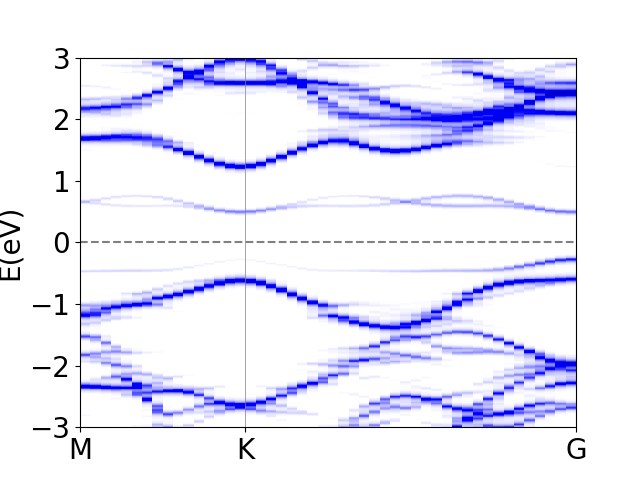
where you can clearly see the defect states in the gap!