Spin-orbit coupling¶

The spin-orbit module calculates spin-orbit band structures non self-consistently. The input is a standard converged GPAW calculation and the module diagonalizes the spin-orbit Hamiltonian in a basis of scalar- relativistic Kohn-Sham eigenstates. Since the spin-obit coupling is largest close to the nucleii, we only consider contributions from inside the PAW augmentation spheres where the all-electron states can be expanded as

\[|\psi_{nk}\rangle= \sum_{ai}\langle\tilde p_i^a|\tilde\psi_{nk}\rangle|\phi_i^a\rangle\]

The full Bloch Hamiltonian in a basis of scalar relativistic states becomes

\[H_{nn'\sigma\sigma'}(k)= \varepsilon_{nk\sigma}\delta_{nn'\sigma\sigma'}+ \langle\psi_{nk\sigma}|H^{SO}(k)|\psi_{n'k\sigma'}\rangle= \varepsilon_{nk\sigma}\delta_{nn'\sigma\sigma'}+ \sum_{ai_1i_2}\langle\tilde\psi_{nk}|\tilde p_{i_1}^a\rangle \langle\phi_{i_1}\sigma|H^{SO}(k)|\phi_{i_2}\sigma'\rangle \langle\tilde p_{i_2}^a|\tilde\psi_{n'k}\rangle\]

where the spinors are chosen along the \(z\) axis as default. Thus, if calc is an instance of the GPAW calculator with converged wavefunctions the spin-orbit coupled states can be obtained with the soc_eigenstates() function which will return an instance of BZWaveFunctions. The eigenvalues are obtained by calling the eigenvalues() method:

from gpaw.spinorbit import soc_eigenstates
soc = soc_eigenstates(calc)
e_km = soc.eigenvalues()

Here e_km is an array of dimension (Nk, 2 * Nb), where Nb is the number of bands and Nk is the number of irreducible k-points. Is is also possible to obtain the eigenstates of the full spin-orbit Hamiltonian as well as the spin character along the z axis. The spin character is defined as

\[s_{mk}\equiv\langle mk|\sigma_z|mk\rangle\]

and is useful for analyzing the degree of spin-orbit induced hybridization between spin up and spin down states. Examples of this will be given below. The implementation is documented in Ref. [1]

gpaw.spinorbit.soc_eigenstates(calc, n1=None, n2=None, scale=1.0, theta=0.0, phi=0.0, eigenvalues=None, occcalc=None, projected=False)[source]¶

Calculate SOC eigenstates.

Parameters:

calc (ASECalculator | GPAW | str | Path) – Calculator GPAW calculator or path to gpw-file.
n1 (int) – int Range of bands to include (n1 <= n < n2). Default is all bands available.
n2 (int) – int Range of bands to include (n1 <= n < n2). Default is all bands available.
scale (float) – float Scale the spinorbit coupling by this amount.
theta (float) – float Angle in degrees.
phi (float) – float Angle in degrees.
eigenvalues (Array3D) – ndarray Optionally use these eigenvalues instead for those from calc. The shape must be: (nspins, nibzkpts, n2 - n1). Units: eV.
occcalc (OccupationNumberCalculator) – Occupation-number calculator. By default, the one from calc will be used.

Returns a BZWaveFunctions object covering the whole BZ.

Band structure of bulk Pt¶

The spin-orbit coupling is strongest for the heavy elements, where the electrons acquire large velocites near the nucleus. We will therefore start with the band structure of bulk Pt, where the spin-orbit coupling gives rise to large corrections. First, we need to do a regular groundstate calculation to obtain the converged density. This is done with the script Pt_gs.py. We then calculate the band structure at fixed density along a certain Brillouin zone path with the script Pt_bands.py. Finally the full spin-orbit coupled bandstructure is calculated and plotted with the following script plot_Pt_bands.py. The spin-orbit calculation takes on the order of a second, while the preceding scripts takes a bit longer and could be parallelized. The band structure without spin-orbit coupling is shown as dashed grey lines. Note that we only plot every second spin-orbit band, since time-reversal symmetry along with inversion symmetry dictates that all bands are two-fold degenerate (you can check this for the present case). The plot is shown below.

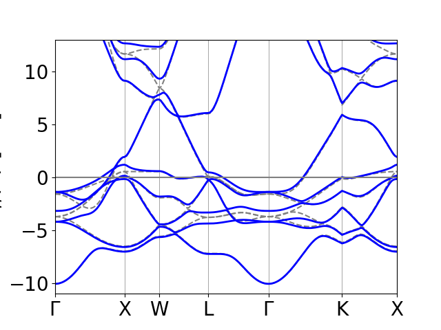
An important property of the spin-orbit interaction is the fact that it can lift degeneracies between states that are protected by symmetry when spin- orbit coupling is absent. This is well-known for the hydrogen atom where the spin-orbit interaction splits the six \(p\) states into two \(j=1/2\) states and four \(j=3/2\) states. In solid state spectra, this splitting often gives rise to avoided crossings at certain point in the Brillouin zone. For example, In the present case, there is a band crossing at \(W\) approximately 8.5 eV above the Fermi level. This degeneracy is lifted by the spin-orbit coupling and the bands become split by 1 eV at this point. Also note that two of the \(d\)-states are degenerate along the entire \(\Gamma-X\) line without spin-orbit coupling, but the degeneracy is lifted when spin-orbit coupling is included.

Band structure of monolayer WS2¶

Things become even more interesting when we consider systems without inversion symmetry, where the spin-orbit coupling may lift the spin-degeneracy. An important class of examples exhibiting this behavior is monolayers of the transition metal dichalcogenides. Here we focus on \(\text{WS}_2\). Again we start by a regular groundstate calculation to obtain the converged density. This is done with the script WS2_gs.py. We then calculate the band structure with the script WS2_bands.py, which also returns a file with the path in k-space and another file with the position of high symmetry points. The spin-orbit coupled bandstructure is calculated and plotted with the script plot_WS2_bands.py. In addition to the eigenvalues, the spin character is now returned as well and displayed as marker color in a scatter plot. The band structure without spin-orbit coupling is again shown as dashed grey lines. The plot is shown below.

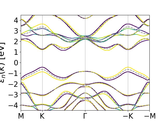
Here, spin is displayed as light yellow and spin down is displayed as dark green. Most places the bands are +1 or -1 signaling that the bands are approximate eigenstates of the spin projection operator along the z axis. Exceptions occur near avoided crossings where the spin-orbit coupling gives rise to strong hybridization between spin up and spin down states. Note also the large spin-orbit splitting (0.44 eV) of the valence bands at \(K\) and \(-K\) and the fact that time-reversal symmetry dictates that the spin projecton is reversed at the two valleys.

Band structure of bulk Fe¶

As another example we consider bcc Fe. Here the spin-orbit coupling breaks the symmetry between Brillouin zone points that are otherwise equivalent. We thus consider two different \(\Gamma-H\) paths. One along the spin projection axis and one orthogonal to it. The scripts for the groundstate Fe_gs.py, bandstructure Fe_bands.py and plotting plot_Fe_bands.py are similar to the previous examples. The result is shown below.

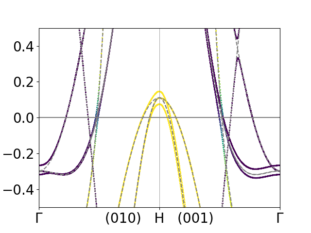
Topological index of Bi2Se3¶

Time-reversal invariant band insulators fall in two distinct topological classes, which can be distinguished by the so-called \(\text{Z}_2\) index \(\nu\). In general, the calculation of the \(\text{Z}_2\) index is a complicated task, but for materials with an inversion center is is easily expressed in terms ofthe parity eigenvalues of occupied states at the parity invariant points in the Brillouin zone. It is given by [2]

\[(-1)^{\nu}=\prod_a\prod_m\xi_m(\Lambda_a)\]

where \(\xi_m\) are the parity eigenvalues of Kramers pairs of occupied bands at the parity invariant points \(\Lambda_a\).

As an example we consider the topological insulator \(\text{Bi}_2\text{Se}_3\). Again the scripts for the groundstate gs_Bi2Se3.py, bandstructure Bi2Se3_bands.py and plotting plot_Bi2Se3_bands.py are similar to the previous examples. The band structure is shown below

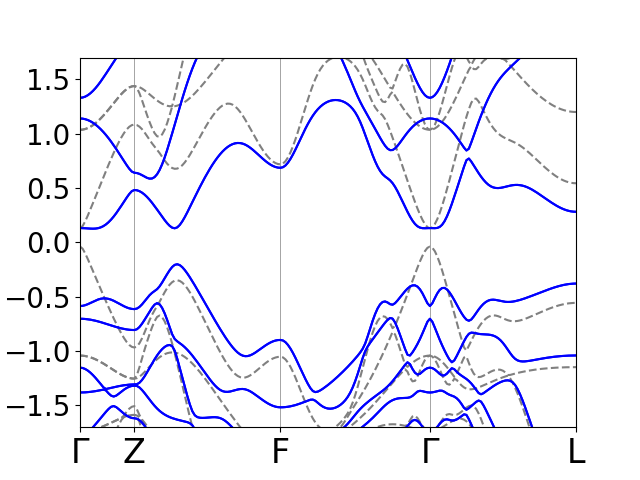
Note the “band inversion” at the \(\Gamma\) point. The spin-orbit coupling essentially bring the bottom of the conduction band below the top of the valence band and opens a gap a the band crossings. We will now calculate the parity eigenvalues at the parity invariant points. In 3D there is 8 such points, but in the present case only 4 are inequivalent. These are calcaluted with the script high_sym.py and the parity eigenvalues are obtained with parity.py. Note that the product of parity eigenvalues at \(\Gamma\) changes from -1 to 1 when spin-orbit coupling is added and the \(\nu\) thus changes from 0 to 1.

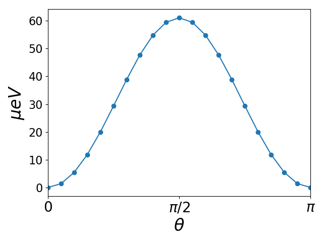
Magnetic anisotropy of hcp Co¶

As a final application of the spinorbit module we will calculate the magnetic anisotropy of hcp Co. The idea is that the direction of spin polarization before spin-orbit coupling is added, can set by the polar and azimutal angles \(\theta\) and \(\phi\). To leading order the spin-orbit induced change in energy as a function of direction is given by the change of occupied eigenvalues. The anisotropy energy per unit cell is typically measured in \(\mu eV\) and for metals, the states close to the Fermi level will be very important. For this reason, we need quite high k-point sampling to converge the calculation. The following script generates the ground state of hcp Co with a dense k-point sampling gs_Co.py. The script anisotropy.py calculates the ground state energy when \(\theta\) takes values on a path from 0 to 180 (easy to hard to easy axes). The results are shown below and was generated with the script plot_anisotropy.py. The curve exhibits a maximum at \(\theta=90\), which is the hard axis. The magnetic anisotropy energy is \(\sim 60 \mu eV\) per unit cell, which agrees well with the experimental value of \(70 \mu eV\).