Tutorial: STM images - Al(111)

Let’s make a 2 layer Al(111) fcc surface using the ase.build.fcc111() function:

from ase.build import fcc111
atoms = fcc111('Al', size=(1, 1, 2))
atoms.center(vacuum=4.0, axis=2)

Now we calculate the wave functions and write them to a file:

from gpaw import GPAW
calc = GPAW(mode='pw',
            kpts=(4, 4, 1),
            symmetry='off',
            txt='al111.txt')
atoms.calc = calc
energy = atoms.get_potential_energy()
calc.write('al111.gpw', 'all')

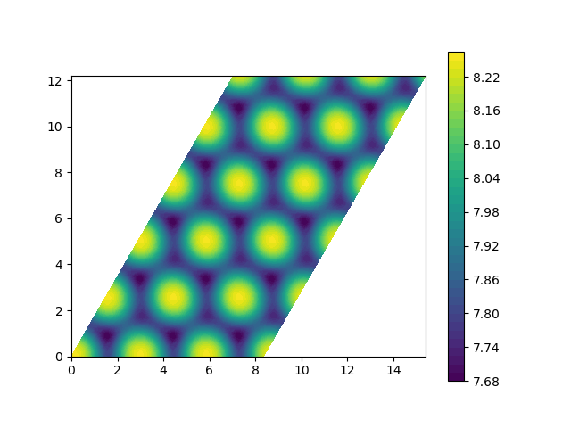
2-d scans

First initialize the STM object and get the averaged current at \(z=8.0\) Å (for our surface, the top layer is at \(z=6.338\) Å):

# web-page: 2d.png, 2d_I.png, line.png, dIdV.png
from ase.dft.stm import STM
from gpaw import GPAW
calc = GPAW('al111.gpw')
atoms = calc.get_atoms()
stm = STM(atoms)
z = 8.0
bias = 1.0
c = stm.get_averaged_current(bias, z)
x, y, h = stm.scan(bias, c, repeat=(3, 5))

From the current we make a scan to get a 2-d array of constant current height and make a contour plot:

import matplotlib.pyplot as plt
plt.gca().axis('equal')
plt.contourf(x, y, h, 40)
plt.colorbar()
plt.savefig('2d.png')

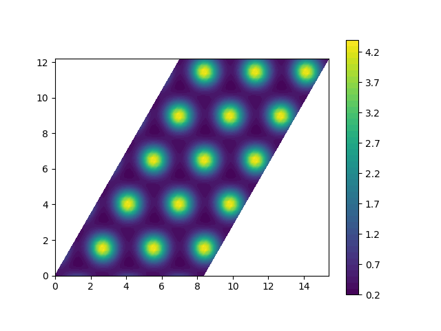
Similarly, we can make a constant height scan (at \(z=8.0\) Å) and plot it:

plt.figure()
plt.gca().axis('equal')
x, y, I = stm.scan2(bias, z, repeat=(3, 5))
plt.contourf(x, y, I, 40)
plt.colorbar()
plt.savefig('2d_I.png')

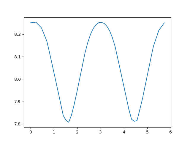
Linescans

Here is how to make a line-scan:

plt.figure()
a = atoms.cell[0, 0]
x, y = stm.linescan(bias, c, [0, 0], [2 * a, 0])
plt.plot(x, y)
plt.savefig('line.png')

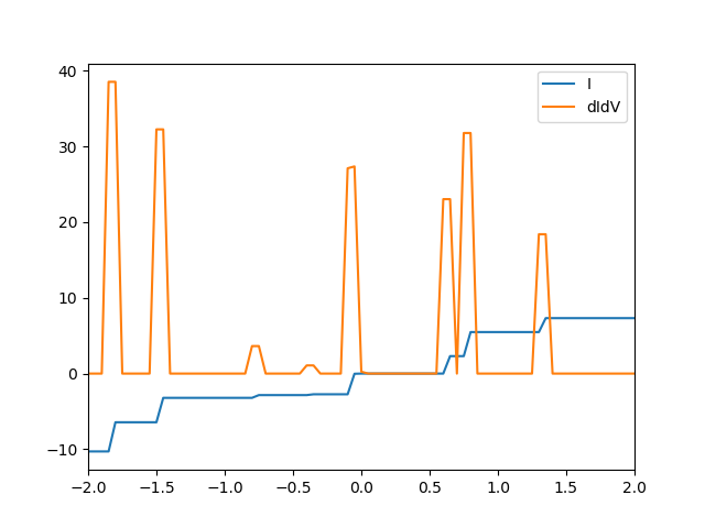
Scanning tunneling spectroscopy

We can also make STS plots (dV/dV curve at specified location; here at \(z=8.0\) Å above atom 0:

plt.figure()
biasstart = -2.0
biasend = 2.0
biasstep = 0.05
bias, I, dIdV = stm.sts(0, 0, z, biasstart, biasend, biasstep)
plt.plot(bias, I, label='I')
plt.plot(bias, dIdV, label='dIdV')
plt.xlim(biasstart, biasend)
plt.legend()
plt.savefig('dIdV.png')