Berry phase calculations
In this tutorial we provide a set of examples of how to calculate various physical properties derived from the \(k\)-space Berry phases.
Spontaneous polarization of tetragonal BaTiO3
As a first example we calculate the spontaneous polarization of the
ferroelectric BaTiO3 in the tetragonal phase. The initial step is to generate
a ground state calculation with wavefunctions. This can be don e with the
script gs_BaTiO3.py. We can then run the script
import numpy as np
from ase.units import _e
from gpaw import GPAW
from gpaw.berryphase import get_polarization_phase
from gpaw.mpi import world

# Create gpw-file with wave functions for all k-points in the BZ:
calc = GPAW('BaTiO3.gpw').fixed_density(symmetry='off')
calc.write('BaTiO3+wfs.gpw', mode='all')

phi_c = get_polarization_phase('BaTiO3+wfs.gpw')
cell_cv = calc.atoms.cell * 1e-10
V = calc.atoms.get_volume() * 1e-30
px, py, pz = (phi_c / (2 * np.pi) % 1) @ cell_cv / V * _e
if world.rank == 0:
    with open('polarization_BaTiO3.out', 'w') as fd:
        print(f'P: {pz} C/m^2', file=fd)
which calculates the polarization. It will take a few minutes on a single CPU, but can also be parallelized. It generates a .json file that contains the polarization and will read if the script is run again. It is thus possible to submit the polarization script and print the polarization by rerunning the script above in the terminal. The calculation adds the contribution from the electrons and the nucleii, which implies that the result is independent of the positions of the atoms relative to the unit cell. The results should be 0.27 \(C/m^2\) for LDA and 0.45 \(C/m^2\) for PBE , which agrees with the values from literature [1]. Technically this approach is incorrect since an adiabatic path between a non-polar reference structure (in this case the cubic phase of BaTiO3) and the polar phase (the tetragonal phase of BaTiO3) is needed in order to properly compute the spontanous polarization [2]. However for BaTiO3 the spontaneous polarization happens to be smaller than the so called polarization quantum, and therefore the approach presented here yields the correct result.
Born effective charges of tetragonal BaTiO3
The Berry phase module can also be used to calculate Born effective charges. They are defined by
where \(u_j^a\) is the position of atom \(a\) in direction \(j\) relative to the equilibrium position and \(P_i\) is the polarization in direction \(i\). Like the case of phonons all atoms are moved in all possible directions and the induced polarization is calculated for each move. For the BaTiO3 structure calculated above the calculation is performed with the script
from gpaw import GPAW
from gpaw.borncharges import borncharges

calc = GPAW('BaTiO3.gpw', txt=None)
borncharges(calc)
Again the results are written to a .json file and the Born effective charges can be viewed with the script
import json
import numpy as np

with open('borncharges-0.01.json') as fd:
    Z_avv = json.load(fd)['Z_avv']
for a, Z_vv in enumerate(Z_avv):
    print(a)
    print(np.round(Z_vv, 2))
Due to symmetry all the tensors are diagonal. Note, however, the large differences between the components for each of the O atoms. The Born effective charges tell us how the atoms are affected by an external electric field.
Topological properties of stanene from parallel transport
We will now demonstrate how the \(k\)-space Berry phases can be applied to extract topological properties of solids. For an isolated band we can calculate the Berry phase
where \(k_i\) is the component of crystal momentum corresponding to \(\mathbf{b}_i\) in reduced coordinates. The Berry phase is only gauge invariant modulo \(2\pi\) and since \(\gamma_1(k_2, k_3)=\gamma_1(k_2+1, k_3)=\gamma_1(k_2,k_3+1)\) modulo \(2\pi\), we can count how many multiples of the \(2\pi\) that \(\gamma_1\) changes while \(k_2\) of \(k_3\) is adiabatically cycled through the Brillouin zone. This is the Chern number, which gives rise to a topological \(\mathbb{Z}\) classification of all two-dimensional insulators. For multiple valence bands the situation is slightly more complicated and one has to introduce the notion of parallel transport to obtain the Berry phases of individual bands. We refer to Ref. [3] for details.
For materials with time-reversal symmetry the Chern number vanishes. Instead,
any insulator in two dimensions can be classified according to a
\(\mathbb{Z}_2\) index \(\nu\) that counts the number of times berry phases
acquire a particular value in half the Brillouin zone modulo two. Below we
give the example of stanene, which is referred to as a quantum spin Hall
insulator due to the non-trivial topology reflected by \(\nu=1\). The ground
state can be set up with the script gs_Sn.py. Afterwards the
Berry phases of all occupied bands are calculated with
import os
from gpaw.berryphase import parallel_transport
from gpaw import GPAW
import gpaw.mpi as mpi

calc = GPAW('gs_Sn.gpw').fixed_density(
    kpts={'size': (7, 200, 1), 'gamma': True},
    symmetry='off',
    txt='Sn_berry.txt')
calc.write('gs_berry.gpw', mode='all')

parallel_transport('gs_berry.gpw', direction=0, name='7x200')

if mpi.world.rank == 0:
    os.system('rm gs_berry.gpw')
Finally the berry phase spectrum can be plottet with
plot_phase.py and the result is shown below.
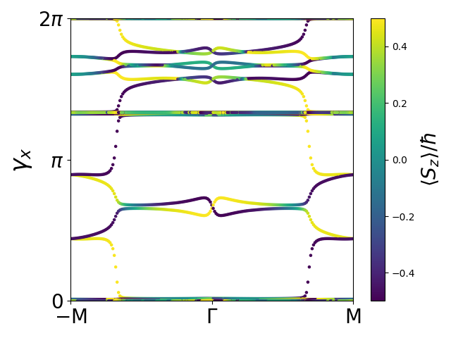
Note the degeneracy of all phases at the time-reversal invariant points \(\Gamma\) and \(M\). Also note that any horizontal line is transversed by an odd number of phases in half the Brillouin zone (for example the \(\Gamma-M\) line). We also display the expectation value of \(S_z\) according to color. This is possible because the individual phases correspond to the first moments of hybrid Wannier functions localized along the \(x\)-direction and these functions have a spinorial structure with a well-defined value of \(\langle S_z\rangle\). [3]
Polarization from from parallel transport
The parallel transport module can also be used to calculate the polarization. Strictly speaking the parallel transport algorithm is not required for the polarization because it involves a trace over occupied bands. Nevertheless, it is reassuring that we obtain the correct polarization from the parallel transport. More importantly, the parallel transport supports spin-orbit coupling and non-collinear magnetism, which the polarization module introduced above does not. The script
import numpy as np
from ase.units import _e
from ase.dft.kpoints import monkhorst_pack
from gpaw import GPAW
from gpaw.berryphase import parallel_transport
from gpaw.mpi import world

phi_i = []

for i in range(8):
    kpts = monkhorst_pack((8, 1, 8))
    kpts += (1 / 16, -3 / 8, 1 / 16)
    kpts += (0, i / 8, 0)

    calc = GPAW('BaTiO3.gpw').fixed_density(symmetry='off', kpts=kpts)
    calc.write('BaTiO3_%s.gpw' % i, mode='all')

    phi_km, S_km = parallel_transport('BaTiO3_%s.gpw' % i, direction=2,
                                      name='BaTiO3_%s' % i, scale=0)

    phi_km[np.where(phi_km < 0.0)] += 2 * np.pi
    phi_i.append(np.sum(phi_km) / len(phi_km))
#    if world.rank == 0:
#        import matplotlib.pyplot as plt
#        for phi_k in phi_km.T:
#            plt.plot(range(8), phi_k, 'o', c='C0')
#        plt.show()

spos_ac = calc.atoms.get_scaled_positions()
Z_a = [10, 12, 6, 6, 6]  # Charge of nucleii

phase = -np.sum(phi_i) / len(phi_i)
phase += 2 * np.pi * np.dot(Z_a, spos_ac)[2]

cell_cv = calc.atoms.cell * 1e-10
V = calc.atoms.get_volume() * 1e-30
pz = (phase / (2 * np.pi) % 1) * cell_cv[2, 2] / V * _e
if world.rank == 0:
    print(f'P: {pz} C/m^2')
    with open('parallel_BaTiO3.out', 'w') as fd:
        print(f'P: {pz} C/m^2', file=fd)
calculates the polarization of BaTiO3 from the parallel transport module. Note that the parallel transport only supports 2D \(k\) grids and we thus loop over slices at fixed \(k_y\) to calculate the polarization. It is also important to realize that the phases at individual points are only defined modulo \(2\pi\) and the phases has to be chosen such that the bands are continuous. The script is seen to exactly reproduce the value of 0.45 \(C/m^2\) found above. Spin-orbit coupling may be switched on by setting scale=1 in the script.