Calculation of electronic band structures
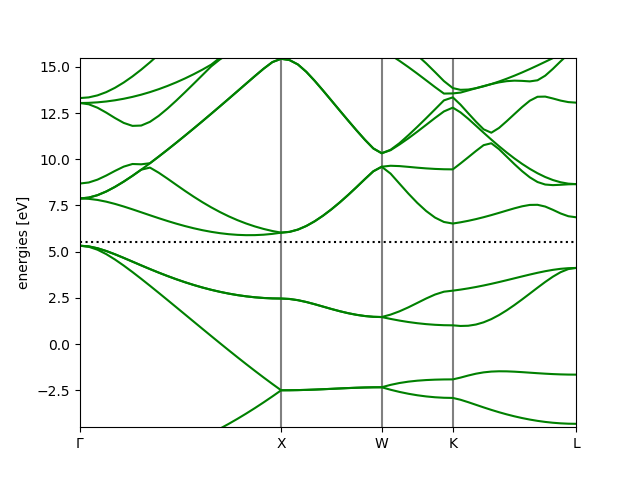
In this tutorial we calculate the electronic band structure of Si along high symmetry directions in the Brillouin zone.
First, a standard ground state calculations is performed and the results are saved to a .gpw file. As we are dealing with small bulk system, plane wave mode is the most appropriate here.
from ase.build import bulk
from gpaw import GPAW, PW, FermiDirac

# Perform standard ground state calculation (with plane wave basis)
si = bulk('Si', 'diamond', 5.43)
calc = GPAW(mode=PW(200),
            xc='PBE',
            kpts=(8, 8, 8),
            random=True,  # random guess (needed if many empty bands required)
            occupations=FermiDirac(0.01),
            txt='Si_gs.txt')
si.calc = calc
si.get_potential_energy()
ef = calc.get_fermi_level()
calc.write('Si_gs.gpw')
Next, we calculate eigenvalues along a high symmetry path in the Brillouin
zone kpts={'path': 'GXWKL', 'npoints': 60}. See
ase.dft.kpoints.special_points for the definition of the special
points for an FCC lattice.
For the band structure calculation, the density is fixed to the previously
calculated ground state density, and as we want to
calculate all k-points, symmetry is not used (symmetry='off').
# Restart from ground state and fix potential:
calc = GPAW('Si_gs.gpw').fixed_density(
    nbands=16,
    symmetry='off',
    kpts={'path': 'GXWKL', 'npoints': 60},
    convergence={'bands': 8})
Finally, the bandstructure can be plotted (using ASE’s band-structure tool
ase.spectrum.band_structure.BandStructure):
bs = calc.band_structure()
bs.plot(filename='bandstructure.png', show=True, emax=10.0)
The full script: bandstructure.py.
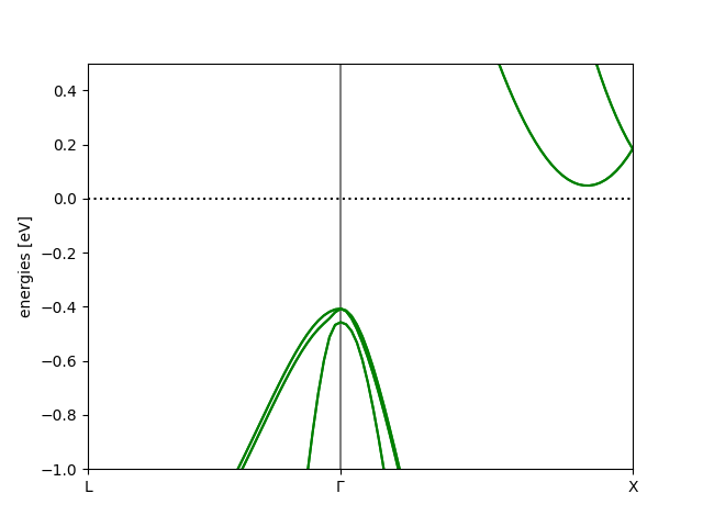
Effect of spin-orbit coupling
Here is a zoom in on the VBM to see the effect of including Spin-orbit coupling:
from ase.build import bulk
from gpaw import GPAW, PW, FermiDirac
import numpy as np

# Non-collinear ground state calculation:
si = bulk('Si', 'diamond', 5.43)
si.calc = GPAW(mode=PW(400),
               xc='LDA',
               experimental={'magmoms': np.zeros((2, 3)),
                             'soc': True},
               kpts=(8, 8, 8),
               symmetry='off',
               occupations=FermiDirac(0.01))
si.get_potential_energy()

bp = si.cell.bandpath('LGX', npoints=100)
bp.plot()

# Restart from ground state and fix density:
calc2 = si.calc.fixed_density(
    nbands=16,
    basis='dzp',
    symmetry='off',
    kpts=bp,
    convergence={'bands': 8})

bs = calc2.band_structure()
bs = bs.subtract_reference()

# Zoom in on VBM:
bs.plot(filename='si-soc-bs.png', show=True, emin=-1.0, emax=0.5)