Density Of States

The density of states is defined by

\[\rho(\varepsilon) = \sum_n \langle\psi_n|\psi_n\rangle \delta(\varepsilon-\varepsilon_n),\]

where \(\varepsilon_n\) is the eigenvalue of the eigenstate \(|\psi_n\rangle\).

Inserting a complete orthonormal basis, this can be rewritten as

\[\begin{split}\begin{array}{rlrl} \rho(\varepsilon) &= \sum_i \rho_i(\varepsilon) ,& \rho_i(\varepsilon) &= \sum_n \langle \psi_n | i \rangle \langle i | \psi_n \rangle \delta(\varepsilon - \varepsilon_n)\\ \rho(\varepsilon) &= \int\!\mathrm{d}r \rho(r, \varepsilon),& \rho(r, \varepsilon) &= \sum_n \langle\psi_n | r \rangle \langle r | \psi_n \rangle \delta(\varepsilon - \varepsilon_n) \end{array}\end{split}\]

using that \(1 = \sum_i | i \rangle\langle i |\) and \(1 = \int\!\mathrm{d}r |r\rangle\langle r|\).

\(\rho_i(\varepsilon)\) is called the projected density of states (PDOS), and \(\rho(r, \varepsilon)\) the local density of states (LDOS).

Notice that an energy integrating of the LDOS multiplied by a Fermi distribution gives the electron density

\[\int\!\mathrm{d}\varepsilon\, n_F(\varepsilon) \rho(r, \varepsilon) = n(r)\]

Summing the PDOS over \(i\) gives the spectral weight of orbital \(i\).

A GPAW calculator gives access to four different kinds of projected density of states:

• Total density of states.

• Molecular orbital projected density of states.

• Atomic orbital projected density of states.

• Wigner-Seitz local density of states.

Each of which are described in the following sections.

Total DOS

The total density of states can be obtained by the GPAW calculator method get_dos(spin=0, npts=201, width=None).

Molecular Orbital PDOS

As shown in the section Density Of States, the construction of the PDOS requires the projection of the Kohn-Sham eigenstates \(|\psi_n\rangle\) onto a set of orthonormal states \(|\psi_{\bar n}\rangle\).

\[\rho_{\bar n}(\varepsilon) = \sum_n | \langle \psi_{\bar n} | \psi_n \rangle |^2 \delta(\varepsilon - \varepsilon_n)\]

The all electron overlaps \(\langle \psi_{\bar n}|\psi_n\rangle\) can be calculated within the PAW formalism from the pseudo wave functions \(|\tilde\psi\rangle\) and their projector overlaps by [1]:

\[\langle \psi_{\bar n} | \psi_n\rangle = \langle \tilde \psi_{\bar n} | \tilde \psi_n \rangle + \sum_a \sum_{i_1i_2} \langle \tilde \psi_{\bar n} | \tilde p_{i_1}^a \rangle \Delta S^a_{i_1i_2} P^a_{ni_2},\]

where \(\Delta S^a_{i_1i_2} = \langle\phi_{i_1}^a|\phi_{i_2}^a\rangle - \langle\tilde\phi_{i_1}^a|\tilde\phi_{i_2}^a\rangle\) is the overlap metric, \(\phi_i^a(r)\), \(\tilde \phi_i^a(r)\), and \(\tilde p^a_i(r)\) are the partial waves, pseudo partial waves and projector functions of atom \(a\) respectively, and \(P^a_{ni} = \langle \tilde p_i^a|\tilde\psi_n\rangle\).

If one chooses the states \(|\psi_{\bar n}\rangle\) as eigenstates of a different reference Kohn-Sham system, with the projector overlaps \(\bar P_{\bar n i}^a\), the PDOS relative to these states can simply be calculated by

\[\langle \psi_{\bar n} | \psi_n\rangle = \langle \tilde \psi_{\bar n} | \tilde \psi_n \rangle + \sum_a \sum_{i_1i_2} \bar P_{\bar n i_1}^{a*} \Delta S^a_{i_1i_2} P^a_{ni_2}.\]

The example below calculates the density of states for CO adsorbed on a Pt(111) slab and the density of states projected onto the gas phase orbitals of CO. The .gpw files can be generated with the script top.py

PDOS script (pdos.py):

# web-page: pdos.png
from gpaw import GPAW, restart
import matplotlib.pyplot as plt

# Density of States
plt.subplot(211)
slab, calc = restart('top.gpw')
e, dos = calc.get_dos(spin=0, npts=2001, width=0.2)
e_f = calc.get_fermi_level()
plt.plot(e - e_f, dos)
plt.axis([-15, 10, None, 4])
plt.ylabel('DOS')

molecule = range(len(slab))[-2:]

plt.subplot(212)
c_mol = GPAW('CO.gpw')
for n in range(2, 7):
    print('Band', n)
    # PDOS on the band n
    wf_k = [kpt.psit_nG[n] for kpt in c_mol.wfs.kpt_u]
    P_aui = [[kpt.P_ani[a][n] for kpt in c_mol.wfs.kpt_u]
             for a in range(len(molecule))]
    e, dos = calc.get_all_electron_ldos(mol=molecule, spin=0, npts=2001,
                                        width=0.2, wf_k=wf_k, P_aui=P_aui)
    plt.plot(e - e_f, dos, label='Band: ' + str(n))
plt.legend()
plt.axis([-15, 10, None, None])
plt.xlabel('Energy [eV]')
plt.ylabel('All-Electron PDOS')
plt.savefig('pdos.png')
plt.show()

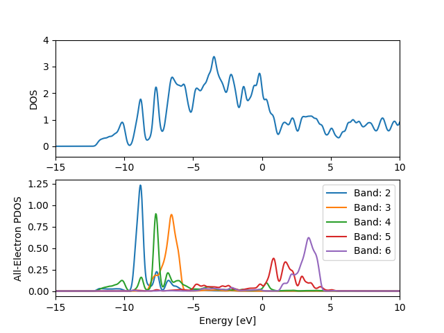
When running the script \(\int d\varepsilon\rho_i(\varepsilon)\) is printed for each spin and k-point. The value should be close to one if the orbital \(\psi_i(r)\) is well represented by an expansion in Kohn-Sham orbitals and thus the integral is a measure of the completeness of the Kohn-Sham system. The bands 7 and 8 are delocalized and are not well represented by an expansion in the slab eigenstates (Try changing range(2,7) to range(2,9) and note the integral is less than one).

The function calc.get_all_electron_ldos() calculates the square modulus of the overlaps and multiply by normalized gaussians of a certain width. The energies are in eV and relative to the average potential. Setting the keyword raw=True will return only the overlaps and energies in Hartree. It is useful to simply save these in a .pickle file since the .gpw files with wave functions can be quite large. The following script pickles the overlaps

Pickle script (p1.py):

from gpaw import GPAW, restart
import pickle

slab, calc = restart('top.gpw')
c_mol = GPAW('CO.gpw')
molecule = range(len(slab))[-2:]
e_n = []
P_n = []
for n in range(c_mol.get_number_of_bands()):
    print('Band: ', n)
    wf_k = [kpt.psit_nG[n] for kpt in c_mol.wfs.kpt_u]
    P_aui = [[kpt.P_ani[a][n] for kpt in c_mol.wfs.kpt_u]
             for a in range(len(molecule))]
    e, P = calc.get_all_electron_ldos(mol=molecule, wf_k=wf_k, spin=0,
                                      P_aui=P_aui, raw=True)
    e_n.append(e)
    P_n.append(P)
pickle.dump((e_n, P_n), open('top.pickle', 'wb'))

Plot PDOS (p2.py):

from ase.units import Hartree
from gpaw import GPAW
from gpaw.utilities.dos import fold
import pickle
import matplotlib.pyplot as plt

e_f = GPAW('top.gpw').get_fermi_level()

e_n, P_n = pickle.load(open('top.pickle', 'rb'))
for n in range(2, 7):
    e, ldos = fold(e_n[n] * Hartree, P_n[n], npts=2001, width=0.2)
    plt.plot(e - e_f, ldos, label='Band: ' + str(n))
plt.legend()
plt.axis([-15, 10, None, None])
plt.xlabel('Energy [eV]')
plt.ylabel('PDOS')
plt.show()

[1]

16. 5. Blöchl, Phys. Rev. B 50, 17953 (1994)

Atomic Orbital PDOS

If one chooses to project onto the all electron partial waves (i.e. the wave functions of the isolated atoms) \(\phi_i^a\), we see directly from the expression of section Molecular Orbital PDOS, that the relevant overlaps within the PAW formalism is

\[\langle \phi^a_i | \psi_n\rangle = \langle \tilde \phi^a_i | \tilde \psi_n \rangle + \sum_{a'} \sum_{i_1i_2} \langle \tilde \phi^a_i | \tilde p_{i_1}^{a'} \rangle \Big(\langle \phi_{i_1}^{a'} | \phi_{i_2}^{a'} \rangle - \langle \tilde \phi_{i_1}^{a'} | \tilde \phi_{i_2}^{a'}\rangle \Big)\langle \tilde p^{a'}_{i_2} | \tilde \psi_n \rangle\]

Using that projectors and pseudo partial waves form a complete basis within the augmentation spheres, this can be re-expressed as

\[\langle \phi^a_i | \psi_n \rangle = P^a_{ni} + \sum_{a' \neq a} \sum_{i_1i_2} \langle \tilde \phi^a_i | \tilde p^{a'}_{i_1} \rangle \Delta S^{a'}_{i_1i_2} P^{a'}_{ni_2}\]

if the chosen orbital index \(i\) correspond to a bound state, the overlaps \(\langle \tilde \phi^a_i | \tilde p^{a'}_{i_1} \rangle\), \(a'\neq a\) will be small, and we see that we can approximate

\[\langle \phi^a_i | \psi_n \rangle \approx \langle \tilde p_i^a | \tilde \psi_n \rangle\]

We thus define an atomic orbital PDOS by

\[\rho^a_i(\varepsilon) = \sum_n |\langle\tilde p_i^a | \tilde \psi_n \rangle |^2 \delta(\varepsilon - \varepsilon_n) \approx \sum_n | \langle \phi_i^a | \psi_n \rangle |^2 \delta(\varepsilon - \varepsilon_n)\]

available from a GPAW calculator from the method get_orbital_ldos(a, spin=0, angular='spdf', npts=201, width=None).

A specific projector function for the given atom can be specified by an integer value for the keyword angular. Specifying a string value for angular, being one or several of the letters s, p, d, and f, will cause the code to sum over all bound state projectors with the specified angular momentum.

The meaning of an integer valued angular keyword can be determined by running:

>>> from gpaw.utilities.dos import print_projectors
>>> print_projectors('Au')

Note that the set of atomic partial waves do not form an orthonormal basis, thus the properties of the introduction are not fulfilled. This PDOS can however be used as a qualitative measure of the local character of the DOS.

An example of how to obtain and plot the d band on atom number 0 of Au, is shown below (see atomic_orbital_gs.py and atomic_orbital_pdos.py):

from ase.build import bulk
from gpaw import GPAW

atoms = bulk('Au')
k = 8
atoms.calc = GPAW(mode='pw',
                  kpts=(k, k, k))
atoms.get_potential_energy()
atoms.calc.write('au.gpw')

import numpy as np
import matplotlib.pyplot as plt
from gpaw import GPAW

calc = GPAW('au.gpw', txt=None)
energy, pdos = calc.get_orbital_ldos(a=0, angular='d')
energy -= calc.get_fermi_level()
I = np.trapz(pdos, energy)
center = np.trapz(pdos * energy, energy) / I
width = np.sqrt(np.trapz(pdos * (energy - center)**2, energy) / I)
plt.plot(energy, pdos)
plt.xlabel('Energy (eV)')
plt.ylabel('d-projected DOS on atom 0')
plt.title(f'd-band center = {center:.1f} eV, d-band width = {width:.1f} eV')
# plt.show()
plt.savefig('ag-ddos.png')

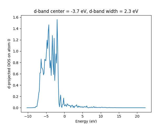
Warning: You should always plot the PDOS before using the calculated center and width to check that it is sensible. The very localized functions used to project onto can sometimes cause an artificial rising tail on the PDOS at high energies. If this happens, you should try to project onto LCAO orbitals instead of projectors, as these have a larger width. This however requires some calculation time, as the LCAO projections are not determined in a standard grid calculation. The projections onto the projector functions are always present, hence using these takes no extra computational effort.

Wigner-Seitz LDOS

(Note: this is currently only implemented for Gamma point calculations, ie. with no k-points.)

For the Wigner-Seitz LDOS, the eigenstates are projected onto the function

\[\begin{split}\theta^a(r) = \begin{cases} 1 & \text{if for all } a' \neq a: |r - R^a| < | r - R^{a'}\\ 0 & \text{otherwise} \end{cases}\end{split}\]

This defines an LDOS:

\[\rho^a(\varepsilon) = \sum_n |\langle \theta^a| \psi_n \rangle|^2 \delta(\varepsilon - \varepsilon_n)\]

Introducing the PAW formalism shows that the weights can be calculated by

\[|\langle \theta^a| \psi_n \rangle|^2 = |\langle \theta^a| \tilde \psi_n \rangle|^2 + \sum_{ij} P^{a*}_{ni} \Delta S^a_{ij} P^a_{nj},\]

This property can be accessed by calc.get_wigner_seitz_ldos(a, spin=0, npts=201, width=None). It represents a local probe of the density of states at atom \(a\). Summing over all atomic sites reproduces the total DOS (more efficiently computed using calc.get_dos). Integrating over energy gives the number of electrons contained in the region ascribed to atom \(a\) (more efficiently computed using calc.get_wigner_seitz_densities(spin). Notice that the domain ascribed to each atom is deduced purely on a geometric criterion. A more advanced scheme for assigning the charge density to atoms is the Bader algorithm (all though the Wigner-Seitz approach is faster).

PDOS on LCAO orbitals

DOS can be also be projected onto the LCAO basis functions. A subspace of the atomic orbitals is required as an input onto which one wants the projected density of states. For example, if the p orbitals of a particular atom in have the indices 41, 42 and 43, and the PDOS is required on the subpspace of these three orbital then an array [41, 42, 43] has to be given as an input for the PDOS calculation.

An example and with explanation is provided below.

LCAO PDOS (see lcaodos_gs.py and lcaodos_plt.py):

# web-page: lcaodos.png
import matplotlib.pyplot as plt
import numpy as np
from ase.io import read
from ase.units import Hartree

from gpaw import GPAW
from gpaw.utilities.dos import RestartLCAODOS, fold


name = 'HfS2'
calc = GPAW(name + '.gpw', txt=None)
atoms = read(name + '.gpw')
ef = calc.get_fermi_level()

dos = RestartLCAODOS(calc)
energies, weights = dos.get_subspace_pdos(range(51))
e, w = fold(energies * Hartree, weights, 2000, 0.1)

e, m_s_pdos = dos.get_subspace_pdos([0, 1])
e, m_s_pdos = fold(e * Hartree, m_s_pdos, 2000, 0.1)
e, m_p_pdos = dos.get_subspace_pdos([2, 3, 4])
e, m_p_pdos = fold(e * Hartree, m_p_pdos, 2000, 0.1)
e, m_d_pdos = dos.get_subspace_pdos([5, 6, 7, 8, 9])
e, m_d_pdos = fold(e * Hartree, m_d_pdos, 2000, 0.1)

e, x_s_pdos = dos.get_subspace_pdos([25])
e, x_s_pdos = fold(e * Hartree, x_s_pdos, 2000, 0.1)
e, x_p_pdos = dos.get_subspace_pdos([26, 27, 28])
e, x_p_pdos = fold(e * Hartree, x_p_pdos, 2000, 0.1)

w_max = []
for i in range(len(e)):
    if (-4.5 <= e[i] - ef <= 4.5):
        w_max.append(w[i])

w_max = np.asarray(w_max)

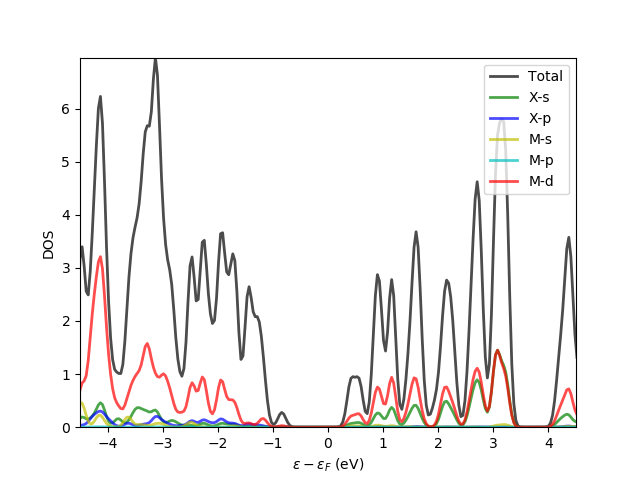
Few comments about the above script. There are 51 basis functions in the calculations and the total density of state (DOS) is calculated by projecting the DOS on all the orbitals.

The projected density of state (PDOS) is calculated for other orbitals as well, for example, s, p and d orbitals of the metal atom and s and p orbitals for the chalcogen atoms. In the subspace of orbitals the basis localized part of the basis functions is not taken into account and only the confined orbital part (larger rc) is chosen.

There is a smarter way of getting the above orbitals in an automated way but it will come later.

Last part of lcaodos_plt.py script:

plt.plot(e - ef, w, label='Total', c='k', lw=2, alpha=0.7)
plt.plot(e - ef, x_s_pdos, label='X-s', c='g', lw=2, alpha=0.7)
plt.plot(e - ef, x_p_pdos, label='X-p', c='b', lw=2, alpha=0.7)
plt.plot(e - ef, m_s_pdos, label='M-s', c='y', lw=2, alpha=0.7)
plt.plot(e - ef, m_p_pdos, label='M-p', c='c', lw=2, alpha=0.7)
plt.plot(e - ef, m_d_pdos, label='M-d', c='r', lw=2, alpha=0.7)

plt.axis(ymin=0., ymax=np.max(w_max), xmin=-4.5, xmax=4.5, )
plt.xlabel(r'$\epsilon - \epsilon_F \ \rm{(eV)}$')
plt.ylabel('DOS')
plt.legend(loc=1)
plt.savefig('lcaodos.png')
plt.show()

WIP

class gpaw.dos.DOSCalculator(wfs, setups=None, cell=None, shift_fermi_level=True)

classmethod from_calculator(filename, soc=False, theta=0.0, phi=0.0, shift_fermi_level=True)

Create DOSCalculator from a GPAW calculation.

filename: str

Name of restart-file or GPAW calculator object.

raw_dos(energies, spin=None, width=0.1)

Calculate density of states.

width: float

Width of Gaussians in eV. Use width=0.0 to use the linear-tetrahedron-interpolation method.

raw_pdos(energies, a, l, m=None, spin=None, width=0.1)

Calculate projected density of states.

a:

Atom index.

l:

Angular momentum quantum number.

m:

Magnetic quantum number. Default is None meaning sum over all m. For p-orbitals, m=0,1,2 translates to y, z and x. For d-orbitals, m=0,1,2,3,4 translates to xy, yz, 3z2-r2, zx and x2-y2.

spin:

Must be 0, 1 or None meaning spin-up, down or total respectively.

width: float

Width of Gaussians in eV. Use width=0.0 to use the linear-tetrahedron-interpolation method.