Calculating band gap using the GLLB-sc functional
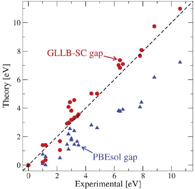
In this tutorial, we calculate the band gaps of semiconductors by using the GLLB-sc functional. [1] The calculation involves correcting the Kohn-Sham band gap with the discontinuity obtained from the response potential. This approach has been shown to improve the band gap description as shown in the figure below taken from [2].
A band gap calculation starts with a usual ground state calculation (here for silicon):
from ase.build import bulk
from gpaw import GPAW, PW, FermiDirac

# Ground state calculation
atoms = bulk('Si', 'diamond', 5.431)
calc = GPAW(mode=PW(200),
            xc='GLLBSC',
            kpts=(7, 7, 7),  # Choose and converge carefully!
            occupations=FermiDirac(0.01),
            txt='gs.out')
atoms.calc = calc
atoms.get_potential_energy()
Then we calculate the discontinuity potential, the discontinuity, and the band gap with the following steps:
# Calculate the discontinuity potential and the discontinuity
homo, lumo = calc.get_homo_lumo()
response = calc.hamiltonian.xc.response
dxc_pot = response.calculate_discontinuity_potential(homo, lumo)
KS_gap, dxc = response.calculate_discontinuity(dxc_pot)

# Fundamental band gap = Kohn-Sham band gap + derivative discontinuity
QP_gap = KS_gap + dxc

print(f'Kohn-Sham band gap:         {KS_gap:.2f} eV')
print(f'Discontinuity from GLLB-sc: {dxc:.2f} eV')
print(f'Fundamental band gap:       {QP_gap:.2f} eV')
Warning
Note that the band edges (HOMO/VBM and LUMO/CBM) are needed as inputs for the discontinuity potential! To get accurate results, both VBM and CBM should be included in the used k-point sampling. See the next example.
This calculation gives for silicon the band gap of 1.05 eV (compare to the experimental value of 1.17 eV [1]).
The accurate values of HOMO/VBM and LUMO/CBM are important for the calculation, and one strategy for evaluating them accurately is to use a band structure calculator that has VBM and CBM at the bandpath:
from ase.build import bulk
from gpaw import GPAW, PW, FermiDirac

# Ground state calculation
atoms = bulk('Si', 'diamond', 5.431)
calc = GPAW(mode=PW(200),
            xc='GLLBSC',
            kpts={'size': (8, 8, 8), 'gamma': True},
            occupations=FermiDirac(0.01),
            txt='gs.out')
atoms.calc = calc
atoms.get_potential_energy()

# Band structure calculation with fixed density
bs_calc = calc.fixed_density(nbands=10,
                             kpts={'path': 'LGXWKL', 'npoints': 60},
                             symmetry='off',
                             convergence={'bands': 8},
                             txt='bs.out')

# Plot the band structure
bs = bs_calc.band_structure().subtract_reference()
bs.plot(filename='bs_si.png', emin=-6, emax=6)
Then we evaluate band edges using bs_calc, the discontinuity potential
using calc, and the discontinuity using bs_calc
(including at least VBM and CBM):
# Get the accurate HOMO and LUMO from the band structure calculator
homo, lumo = bs_calc.get_homo_lumo()

# Calculate the discontinuity potential using the ground state calculator and
# the accurate HOMO and LUMO
response = calc.hamiltonian.xc.response
dxc_pot = response.calculate_discontinuity_potential(homo, lumo)

# Calculate the discontinuity using the band structure calculator
bs_response = bs_calc.hamiltonian.xc.response
KS_gap, dxc = bs_response.calculate_discontinuity(dxc_pot)

# Fundamental band gap = Kohn-Sham band gap + derivative discontinuity
QP_gap = KS_gap + dxc

print(f'Kohn-Sham band gap:         {KS_gap:.2f} eV')
print(f'Discontinuity from GLLB-sc: {dxc:.2f} eV')
print(f'Fundamental band gap:       {QP_gap:.2f} eV')
Warning
Note that also when using the band structure calculator, one needs to make sure that both VBM and CBM exists at the bandpath!
Also this calculation gives for silicon the band gap of 1.05 eV (compare to the experimental value of 1.17 eV [1]).
Note
The first, simple approach would give very different results if
kpts=(7, 7, 7) would be changed to
kpts={'size': (8, 8, 8), 'gamma': True} (try it out!).
When using the second approach with a suitable band structure calculator
for obtaining VBM and CBM, issues with different k-point samplings
can often be avoided.
The full scripts: gllbsc_si_simple.py and
gllbsc_si_band_edges.py.
Spin-polarized GLLB-SC
Spin-polarized GLLB-SC is currently implemented to svn trunk. However there are some convergence issues releated to fermi smearing and the reference energy of highest orbital. Also some parts are still untested. The code will be improved to robust version soon, but in the meantime please contact mikael.kuisma@tut.fi before using.