Charge Analysis
Bader
Henkelman et al. have implemented a fast and robust algorithm for calculating the electronic charges on individual atoms in molecules or crystals, based on the Bader partitioning scheme [Bader]. In that method, the analysis is based purely on the electron density. The partitioning of the density is determined according to its zero-flux surfaces. Details of their implementation can be found in [Tang]. The program is freely available at https://theory.cm.utexas.edu/henkelman/research/bader/ where you will also find a description of the method.
The algorithm is well suited for large solid state physical systems, as well as large biomolecular systems. The computational time depends only on the size of the 3D grid used to represent the electron density, and scales linearly with the total number of grid points. As the accuracy of the method depends on the grid spacing, it is recommended to check for convergence in this parameter (which should usually by smaller than the default value).
The program takes cube input files. It does not support units, and assumes atomic units for the density (\(\text{bohr}^{-3}\)).
A simple Python script for making a cube file containing the electron density of the water molecule, ready for the Bader program, could be:
from ase.build import molecule
from ase.io import write
from ase.units import Bohr
from gpaw import GPAW
from gpaw.analyse.hirshfeld import HirshfeldPartitioning

atoms = molecule('H2O')
atoms.center(vacuum=3.5)
atoms.calc = GPAW(mode='fd', h=0.17, txt='h2o.txt')
atoms.get_potential_energy()

# write Hirshfeld charges out
hf = HirshfeldPartitioning(atoms.calc)
for atom, charge in zip(atoms, hf.get_charges()):
    atom.charge = charge
# atoms.write('Hirshfeld.traj') # XXX Trajectory writer needs a fix
atoms.copy().write('Hirshfeld.traj')

# create electron density cube file ready for bader
rho = atoms.calc.get_all_electron_density(gridrefinement=4)
write('density.cube', atoms, data=rho * Bohr**3)
One can also use get_pseudo_density() but it is
better to use the get_all_electron_density()
method as it will create a normalized electron density with all the electrons.
Note that it is strongly recommended to use version 0.26b or higher of the program, and the examples below refer to this version.
See also
Example: The water molecule
The following example shows how to do Bader analysis for a water molecule.
First do a ground state calculation, and save the density as a cube file:
from ase.build import molecule
from ase.io import write
from ase.units import Bohr
from gpaw import GPAW
from gpaw.analyse.hirshfeld import HirshfeldPartitioning

atoms = molecule('H2O')
atoms.center(vacuum=3.5)
atoms.calc = GPAW(mode='fd', h=0.17, txt='h2o.txt')
atoms.get_potential_energy()

# write Hirshfeld charges out
hf = HirshfeldPartitioning(atoms.calc)
for atom, charge in zip(atoms, hf.get_charges()):
    atom.charge = charge
# atoms.write('Hirshfeld.traj') # XXX Trajectory writer needs a fix
atoms.copy().write('Hirshfeld.traj')

# create electron density cube file ready for bader
rho = atoms.calc.get_all_electron_density(gridrefinement=4)
write('density.cube', atoms, data=rho * Bohr**3)
Then analyse the density cube file by running (use bader -h for a description of the possible options):
$ bader -p all_atom -p atom_index density.cube
This will produce a number of files. The ACF.dat file, contains a summary of the Bader analysis:
    #         X           Y           Z        CHARGE     MIN DIST    ATOMIC VOL
 --------------------------------------------------------------------------------
    1      6.6140      8.0564      7.7409      9.1505      1.3438   2025.9776
    2      6.6140      9.4987      6.6140      0.4248      0.3015    520.7426
    3      6.6140      6.6140      6.6140      0.4248      0.3015    512.9093
 --------------------------------------------------------------------------------
   NUMBER OF ELECTRONS:       10.00004
Revealing that 0.58 electrons have been transferred from each Hydrogen atom to the Oxygen atom.
The BvAtxxxx.dat files, are cube files for each Bader volume, describing the density within that volume. (I.e. it is just the original cube file, truncated to zero outside the domain of the specific Bader volume).
AtIndex.dat is a cube file with an integer value at each grid point, describing which Bader volume it belongs to.
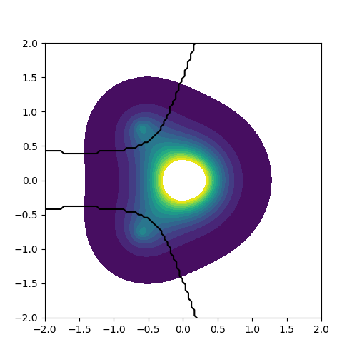
The plot below shows the dividing surfaces of the Hydrogen Bader
volumes. This was achieved by plotting a contour surface of
AtIndex.dat at an isovalue of 1.5 (see plot.py).
Hirshfeld
Another charge analysis is possible by using the Hirshfeld [Hirsh] charges as are written out in the example above.
from ase import io
from ase.io.bader import attach_charges

hirsh = io.read('Hirshfeld.traj')

bader = hirsh.copy()
attach_charges(bader)

print('atom Hirshfeld Bader')
for ah, ab in zip(hirsh, bader):
    assert ah.symbol == ab.symbol
    print(f'{ah.symbol:4s} {ah.charge:9.2f} {ab.charge:5.2f}')
R. F. W. Bader. Atoms in Molecules: A Quantum Theory. Oxford University Press, New York, 1990.
W. Tang, E. Sanville, G. Henkelman. A grid-based Bader analysis algorithm without lattice bias. J. Phys.: Compute Mater. 21, 084204 (2009).
Hirshfeld, Theor. Chim. Acta 44, 129 (1977).