Exact exchange ¶

Currently we have two implementations of exact exchange:

Finite-difference mode implementation: hybrid.py. Can handle Gamma-point only calculations self-consistently (for molecules and large cells). No forces.
Plane-wave mode implementation: . Handles k-points, exploits symmetries and calculates forces.

Contents

Exact exchange
- Self-consistent finite-difference implementation
- Non self-consistent plane-wave implementation

Self-consistent finite-difference implementation ¶

The current implementation lacks the following features:

Support for periodic systems. Actually, the code won’t complain, but the results have not been tested.
Support for k-point sampling. No consideration has been made as to multiple k-points, or even comlplex wave functions, so this definitely won’t work.
Forces. Force evaluations when including (a fraction of -) the fock operator in the xc-functional has been implemented, but has not been tested.
Speed. Inclusion of Fock exchange is exceedingly slow. The bottleneck is solving the poisson integrals of the Fock operator, which is currently done using an iterative real-space solver with a zero initial guess for the potential at each SCF cycle. This should be optimized.

One way to speed up an exact-exchange (or hybrid) calculation is to use the coarse grid (used for wave functions) instead of the finegrid (used for for densities) for the Fock potentials. This should give a speed-up factor of 8. This can be specified in the xc keyword like in this example test_coarse.py

Parallelization using domain decomposition is fully supported.

The Fock operator can be used to do the hybrid functional PBE0, and of course, Hartree-Fock type EXX. These are accessed by setting the xc keyword to PBE0 or EXX respectively.

The following functionals are suppported:

Functional	Type	Reference
EXX	Global
PBE0	Global	[AB98]
B3LYP	Global	[Ba94]
CAMY-B3LYP	RSF-LR	[SZ12]
CAMY-BLYP	RSF-LR	[AT08]
CAMY-B3LYP	RSF-LR	[SZ12]
LCY-BLYP	RSF-LR	[SZ12]
LCY-PBE	RSF-LR	[SZ12]

Here “Global” denotes global hybrids, which use the same percentage of Hartree-Fock exchange for every point in space, while “RSF-SR” and “RSF-LR” denotes range-separated functionals which mix the fraction of Hartree-Fock and DFT exchange based on the spatial distance between two points, where for a “RSF-SR” the amount of Hartree-Fock exchange decrease with the distance and increase for a “RSF-LR”. See Range separated functionals (RSF) for more detailed information on RSF(-LR).

A thesis on the implementation of EXX in the PAW framework, and the specifics of the GPAW project can be seen on the reports presentations and theses page.

A comparison of the atomization energies of the g2-1 test-set calculated in VASP, Gaussian03, and GPAW is shown in the below two figures for the PBE and the PBE0 functional respectively.

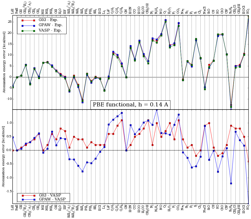
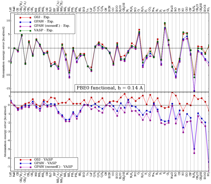
In the last figure, the curve marked GPAW (nonself.) is a non- selfconsistent PBE0 calculation using self-consistent PBE orbitals.

It should be noted, that the implementation lacks an optimized effective potential. Therefore the unoccupied states utilizing EXX as implemented in GPAW usually approximate (excited) electron affinities. Therefore calculations utilizing Hartree-Fock exchange are usually a bad basis for the calculation of optical excitations by lrTDDFT. As a remedy, the improved virtual orbitals (IVOs, [HA71]) were implemented. The requested excitation basis can be chosen by the keyword excitation and the state by excited where the state is counted from the HOMO downwards:

"""Calculate the excitation energy of NaCl by an RSF using IVOs."""
from ase.build import molecule
from ase.units import Hartree
from gpaw import GPAW, setup_paths
from gpaw.mpi import world
from gpaw.occupations import FermiDirac
from gpaw.test import equal, gen
from gpaw.eigensolvers import RMMDIIS
from gpaw.cluster import Cluster
from gpaw.lrtddft import LrTDDFT

h = 0.3  # Gridspacing
e_singlet = 4.3
e_singlet_lr = 4.3

if setup_paths[0] != '.':
    setup_paths.insert(0, '.')

gen('Na', xcname='PBE', scalarrel=True, exx=True, yukawa_gamma=0.40)
gen('Cl', xcname='PBE', scalarrel=True, exx=True, yukawa_gamma=0.40)

c = {'energy': 0.005, 'eigenstates': 1e-2, 'density': 1e-2}
mol = Cluster(molecule('NaCl'))
mol.minimal_box(5.0, h=h)
calc = GPAW(txt='NaCl.txt', xc='LCY-PBE:omega=0.40:excitation=singlet',
            eigensolver=RMMDIIS(), h=h, occupations=FermiDirac(width=0.0),
            spinpol=False, convergence=c)
mol.calc = calc
mol.get_potential_energy()
(eps_homo, eps_lumo) = calc.get_homo_lumo()
e_ex = eps_lumo - eps_homo
equal(e_singlet, e_ex, 0.15)
calc.write('NaCl.gpw')

lr = LrTDDFT(calc, txt='LCY_TDDFT_NaCl.log',
             restrict={'istart': 6, 'jend': 7}, nspins=2)
lr.write('LCY_TDDFT_NaCl.ex.gz')
if world.rank == 0:
    lr2 = LrTDDFT.read('LCY_TDDFT_NaCl.ex.gz')
    lr2.diagonalize()
    ex_lr = lr2[1].get_energy() * Hartree
    equal(e_singlet_lr, e_singlet, 0.05)

Support for IVOs in lrTDDFT is done along the work of Berman and Kaldor [BK79].

If the number of bands in the calculation exceeds the number of bands delivered by the datasets, GPAW initializes the missing bands randomly. Calculations utilizing Hartree-Fock exchange can only use the RMM-DIIS eigensolver. Therefore the states might not converge to the energetically lowest states. To circumvent this problem on can made a calculation using a semi-local functional like PBE and uses this wave-functions as a basis for the following calculation utilizing Hartree-Fock exchange as shown in the following code snippet which uses PBE0 in conjuncture with the IVOs:

"""Test calculation for unoccupied states using IVOs."""

from ase.build import molecule
from gpaw.cluster import Cluster
from gpaw import GPAW, KohnShamConvergenceError, FermiDirac
from gpaw.eigensolvers import CG, RMMDIIS

calc_parms = [
    {'xc': 'PBE0:unocc=True',
     'eigensolver': RMMDIIS(niter=5),
     'convergence': {
         'energy': 0.005,
         'bands': -2,
         'eigenstates': 1e-4,
         'density': 1e-3}},
    {'xc': 'PBE0:excitation=singlet',
     'convergence': {
         'energy': 0.005,
         'bands': 'occupied',
         'eigenstates': 1e-4,
         'density': 1e-3}}]


def calc_me(atoms, nbands):
    """Do the calculation."""
    molecule_name = atoms.get_chemical_formula()
    atoms.set_initial_magnetic_moments([-1.0, 1.0])
    fname = '.'.join([molecule_name, 'PBE-SIN'])
    calc = GPAW(h=0.25,
                xc='PBE',
                eigensolver=CG(niter=5),
                nbands=nbands,
                txt=fname + '.log',
                occupations=FermiDirac(0.0, fixmagmom=True),
                convergence={
                    'energy': 0.005,
                    'bands': nbands,
                    'eigenstates': 1e-4,
                    'density': 1e-3})
    atoms.calc = calc
    try:
        atoms.get_potential_energy()
    except KohnShamConvergenceError:
        pass
    if calc.scf.converged:
        for calcp in calc_parms:
            calc.set(**calcp)
            try:
                calc.calculate(system_changes=[])
            except KohnShamConvergenceError:
                break
        if calc.scf.converged:
            calc.write(fname + '.gpw', mode='all')


loa = Cluster(molecule('NaCl'))
loa.minimal_box(border=6.0, h=0.25, multiple=16)
loa.center()
loa.translate([0.001, 0.002, 0.003])
nbands = 25
calc_me(loa, nbands)

Non self-consistent plane-wave implementation ¶

gpaw.hybrids.energy.non_self_consistent_energy(calc, xcname, ftol=1e-09)[source]¶

Calculate non self-consistent energy for Hybrid functional.

Based on a self-consistent DFT calculation (calc). EXX integrals involving states with occupation numbers less than ftol are skipped.

>>> energies = non_self_consistent_energy('<gpw-file>',
...                                       xcname='HSE06')
>>> e_hyb = energies.sum()

The correction to the self-consistent energy will be energies[1:].sum().

The returned energy contributions are (in eV):

DFT total free energy (not extrapolated to zero smearing)
minus DFT XC energy
Hybrid semi-local XC energy
EXX core-core energy
EXX core-valence energy
EXX valence-valence energy

gpaw.hybrids.eigenvalues.non_self_consistent_eigenvalues(calc, xcname, n1=0, n2=0, kpt_indices=None, snapshot=None, ftol=1e-09)[source]¶

Calculate non self-consistent eigenvalues for a hybrid functional.

Based on a self-consistent DFT calculation (calc). Only eigenvalues n1 to n2 - 1 for the IBZ indices in kpt_indices are calculated (default is all bands and all k-points). EXX integrals involving states with occupation numbers less than ftol are skipped. Use snapshot=’name.json’ to get snapshots for each k-point finished.

Returns three (nspins, nkpts, n2 - n1)-shaped ndarrays with contributions to the eigenvalues in eV:

>>> nsceigs = non_self_consistent_eigenvalues
>>> eig_dft, vxc_dft, vxc_hyb = nsceigs('<gpw-file>', xcname='PBE0')
>>> eig_hyb = eig_dft - vxc_dft + vxc_hyb

See this tutorial: PBE0 calculations for bulk silicon.

Here is an example:

"""EXX hydrogen atom.

Compare self-consistent EXX calculation with non self-consistent
EXX calculation on top of LDA.
"""
from ase import Atoms
from ase.units import Ry
from gpaw import GPAW, PW
from gpaw.hybrids.eigenvalues import non_self_consistent_eigenvalues
from gpaw.hybrids.energy import non_self_consistent_energy

atoms = Atoms('H', magmoms=[1.0])
atoms.center(vacuum=5.0)

# Self-consistent calculation:
atoms.calc = GPAW(mode=PW(600),
                  xc='EXX:backend=pw')
eexx = atoms.get_potential_energy() + atoms.calc.get_reference_energy()

# Check energy
eexxref = -1.0 * Ry
assert abs(eexx - eexxref) < 0.001

# ... and eigenvalues
eig1, eig2 = (atoms.calc.get_eigenvalues(spin=spin)[0] for spin in [0, 1])
eigref1 = -1.0 * Ry
eigref2 = ...  # ?
assert abs(eig1 - eigref1) < 0.03
# assert abs(eig2 - eigref2) < 0.03

# LDA:
atoms.calc = GPAW(mode=PW(600),
                  xc='LDA')
atoms.get_potential_energy()

# Check non self-consistent eigenvalues
result = non_self_consistent_eigenvalues(atoms.calc,
                                         'EXX',
                                         snapshot='h-hse-snapshot.json')
eiglda, vlda, vexx = result
eig1b, eig2b = (eiglda - vlda + vexx)[:, 0, 0]
assert abs(eig1b - eig1) < 0.04
assert abs(eig2b - eig2) < 1.1

# ... and energy
energies = non_self_consistent_energy(atoms.calc, 'EXX')
eexxb = energies.sum() + atoms.calc.get_reference_energy()
assert abs(eexxb - eexx) < 0.03

class gpaw.xc.exx.EXX(gs, xc=None, kpts=None, bands=None, ecut=None, stencil=2, omega=None, world=<gpaw.mpi._Communicator object>, txt=<_io.TextIOWrapper name='<stdout>' mode='w' encoding='utf-8'>, timer=None)[source]¶

Non self-consistent hybrid functional calculations.

Eigenvalues and total energy can be calculated.

calc: str or PAW object: GPAW calculator object or filename of saved calculator object.
xc: str: Name of functional. Use one of EXX, PBE0, HSE03, HSE06 or B3LYP. Default is EXX.
kpts: list of in or list of list of int: List of indices of the IBZ k-points to calculate the quasi particle energies for. Default is all k-points. One can also specify the coordinates of the k-point. As an example, Gamma and X for an FCC crystal would be: kpts=[[0, 0, 0], [1 / 2, 1 / 2, 0]].
bands: tuple of two ints: Range of band indices, like (n1, n2), to calculate the quasi particle energies for. Bands n where n1<=n<n2 will be calculated. Note that the second band index is not included. Default is all occupied bands.
ecut: float: Plane wave cut-off energy in eV. Default it the same as was used for the ground-state calculations.

calculate(restart=None)[source]¶

Do the calculation.

restart_filename: str or Path: Name of restart json-file. Allows for incremental calculation of eigenvalues.

AB98: C. Adamo and V. Barone. Toward Chemical Accuracy in the Computation of NMR Shieldings: The PBE0 Model.. Chem. Phys. Lett. 298.1 (11. Dec. 1998), S. 113–119.
Ba94: V. Barone. Inclusion of Hartree–Fock exchange in density functional methods. Hyperfine structure of second row atoms and hydrides. Jour. Chem. Phys. 101.8 (1994), S. 6834–6838.
BK79: M. Berman and U. Kaldor. Fast calculation of excited-state potentials for rare-gas diatomic molecules: Ne2 and Ar2. Chem. Phys. 43.3 (1979), S. 375–383.
HA71: S. Huzinaga and C. Arnau. Virtual Orbitals in Hartree–Fock Theory. II. Jour. Chem. Phys. 54.5 (1. Ma. 1971), S. 1948–1951.

Exact exchange¶

Self-consistent finite-difference implementation¶

Non self-consistent plane-wave implementation¶

Exact exchange ¶

Self-consistent finite-difference implementation ¶

Non self-consistent plane-wave implementation ¶