Density Mixing
Pulay Mixing
The density is updated using Pulay-mixing [1], [2].
Pulay mixing (or direct inversion of the iterative subspace (DIIS)) attempts to find a good approximation of the final solution as a linear combination of a set of trial vectors \(\{n^i\}\) generated during an iterative solution of a problem. If the error associated with a given solution is given as \(\{R^i\}\) then Pulay mixing assumes that the error of a linear combination of the trail vectors is given as the same linear combination of errors
The norm \(R^{i+1}\) is thus given as
where elements of the matrix is given as \(\bar{\bar{R}}_{ij}=\langle R_{i}|R_{j}\rangle\). The norm can thus be minimized by solving
In density mixing the error of a given input density is given as
The original Pulay mixing only uses \(n_i^{out}\) to calculate the errors and thereby the mixing parameters. To more efficiently cover solution space it can be an advantage to include them with a certain weight, given as the input parameter \(\beta\).
Special Metric
Convergence is improved by an optimized metric \(\hat{M}\) for calculation of scalar products in the mixing scheme, \(\langle A | B \rangle _s = \langle A | \hat{M} | B \rangle\), where \(\langle \rangle _s\) is the scalar product with the special metric and \(\langle \rangle\) is the usual scalar product. The metric is based on the rationale that contributions for small wave vectors are more important than contributions for large wave vectors [2]. Using a metric that weighs short wave density changes more than long wave changes can reduce charge sloshing significantly.
It has been found [2] that the metric
is particularly useful (\(w\) is a suitably chosen weight).
This is easy to apply in plane wave codes, as it is local in reciprocal space. Expressed in real space, this metric is
As this is fully nonlocal in real space, it would be very costly to apply. Instead we use a semilocal stencil with only three nearest neighbors:
which corresponds to the reciprocal space metric
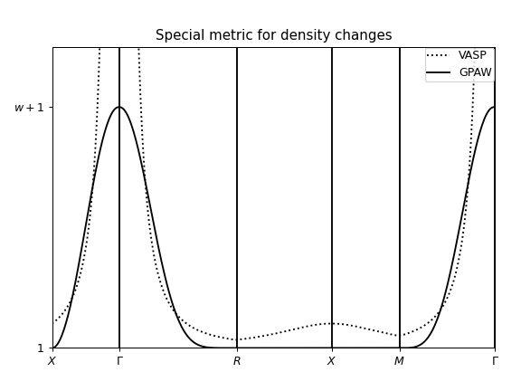
With the nice property that it is a monotonously decaying function from \(f_q = w + 1\) at \(q = 0\) to \(f_q = 1\) anywhere at the zone boundary in reciprocal space.
A comparison of the two metrics is displayed in the figure below
Specifying a Mixing Scheme in GPAW
Specifying the mixing scheme and metric is done using the mixer
keyword of the GPAW calculator:
from gpaw import GPAW, Mixer
calc = GPAW(..., mixer=Mixer(beta=0.05, nmaxold=5, weight=50.0), ...)
which is the recommended value if the default fails to converge.
The class Mixer indicates one of the possible mixing schemes. The
Pulay mixing can be based on:
The spin densities separately,
Mixer(This will not work for a spinpolarized system, unless the magnetic moment is fixed)The total density,
MixerSum2Spin channels separately for the density matrices, and the summed channels for the pseudo electron density,
MixerSumThe total density and magnetization densities separately,
MixerDif
Where the magnetization density is the difference between the two spin densities.
All mixer classes takes the arguments (beta=0.25, nmaxold=3,
weight=50.0). In addition, the MixerDif also takes
the arguments (beta_m=0.7, nmaxold_m=2,
weight_m=10.0) which is the corresponding mixing parameters for the
magnetization density.
Here beta is the linear mixing coefficient, nmaxold is the
number of old densities used, and weight is the
weight used by the metric, if any.
MixerDif seems to be a good choice for spin polarized molecules. MixerSum is sometimes better for bulk systems.