Direct Minimization Methods

Direct minimization methods are an alternative to self-consistent field eigensolvers avoiding density mixing and diagonalization of the Kohn-Sham Hamiltonian matrix.

PW and FD mode

The energy is minimized w.r.t. orbitals subject to orthonomality constraints

\[E_0 = \min_{{\bf\Psi} {\bf \Psi^\dagger} = I} E[{\bf\Psi}].\]

Orbitals are updated at each step according to iteratives:

\[{\bf\Psi}^{(k+1)} \leftarrow {\bf\Psi}^{(k)} + \alpha {\bf V}^{(k)},\]

where search direction, \({\bf V}^{(k)}\), is calculated according to L-BFGS algorithm and projected on the tangent space to orbitals. After each iteration orthonormalization procedure is applied to satify orthonormality constriants. For details of the implementation see Ref. [1]

Example

import numpy as np
from ase import Atoms
from gpaw import GPAW
from gpaw.directmin.etdm_fdpw import FDPWETDM

# Water molecule:
d = 0.9575
t = np.pi / 180 * 104.51
H2O = Atoms('OH2',
            positions=[(0, 0, 0),
                       (d, 0, 0),
                       (d * np.cos(t), d * np.sin(t), 0)])
H2O.center(vacuum=5.0)

calc = GPAW(mode='pw',
            eigensolver=FDPWETDM(converge_unocc=False),
            mixer={'backend': 'no-mixing'},
            occupations={'name': 'fixed-uniform'},
            spinpol=True)
H2O.set_calculator(calc)
H2O.get_potential_energy()

If you want to converge the unoccupied orbitals too then set:

• converge_unocc=True.

LCAO mode

Exponential Transformation Direct Minimization

The orbitals are expanded into a finite basis set:

\[\phi_{i} ({\bf r}) = \sum_{\mu=1..M} O_{\mu i} \chi_{\mu}({\bf r}), \quad i = 1 .. M\]

and the energy needs to be minimized with respect to the expansion coefficients subject to orthonormality constraints:

\[E_0 = \min_{O^{\dagger}SO = I} E\left(O\right)\]

If we have some orthonormal reference orbitals with known coefficient matrix (c.m.) \(C\), then any c.m. \(O\) can be obtained from the reference c.m. \(C\) by some unitary transformation:

\[O = C U\]

where U is a unitary matrix. Thus, the objective is to find the unitary matrix that transforms the reference c.m. into an optimal c.m., minimizing the energy of the electronic system. A unitary matrix can be parametrized as the exponential of a skew-hermitian matrix \(A\):

\[U = \exp(A)\]

This parametrisation is advantageous since the orthonormality constraints are automatically satisfied:

\[UU^{\dagger} = \exp(A)\exp(A^{\dagger}) = \exp(A)\exp(-A) = I\]

If the reference c.m. is fixed, then the energy is a function of \(A\):

\[F\left(A\right) = E\left(C e^A \right)\]

Skew-hermitian matrices form a linear space and, therefore, conventional unconstrained minimization algorithms can be applied to minimize the energy with respect to \(A\).

Example

To run an LCAO calculation with direct minimization, it is necessary to specify the following in the calculator:

• nbands='nao'. Ensures that the number of bands used in the calculation is equal to the number of atomic orbitals.

• mixer={'backend': 'no-mixing'}. No density mixing.

• occupations={'name': 'fixed-uniform'}. Uniform distribution of the occupation numbers (same number of occupied bands for each k-point per spin).

Here is an example of how to run a calculation with direct minimization in LCAO:

from gpaw import GPAW, LCAO
from ase import Atoms
import numpy as np
from gpaw.directmin.etdm_lcao import LCAOETDM
# Water molecule:
d = 0.9575
t = np.pi / 180 * 104.51
H2O = Atoms('OH2',
            positions=[(0, 0, 0),
                       (d, 0, 0),
                       (d * np.cos(t), d * np.sin(t), 0)])
H2O.center(vacuum=5.0)

H2O.calc = GPAW(
    mode=LCAO(),
    basis='dzp',
    eigensolver=LCAOETDM(
        searchdir_algo={'name': 'l-bfgs-p', 'memory': 10}),
    occupations={'name': 'fixed-uniform'},
    mixer={'backend': 'no-mixing'},
    nbands='nao')

H2O.get_potential_energy()

As one can see, it is possible to specify the amount of memory used in the L-BFGS algorithm. The larger the memory, the fewer iterations required to reach convergence. Default value is 3. One cannot use a memory larger than the number of iterations after which the reference orbitals are updated to the canonical orbitals (specified by the keyword update_ref_orbs_counter in LCAOETDM, default value is 20).

Important: The exponential matrix is calculated here using the SciPy function expm. In order to obtain good performance, please make sure that your SciPy library is optimized. Otherwise see Implementation Details.

When all occupied orbitals of a given spin channel have the same occupation number, as in the example above, the functional is unitary invariant and a more efficient algorithm for computing the matrix exponential should be used (see also Implementation Details):

calc = GPAW(eigensolver=LCAOETDM(matrix_exp='egdecomp-u-invar',
                                 representation='u-invar'),
            ...)

Performance

G2 Molecular Set

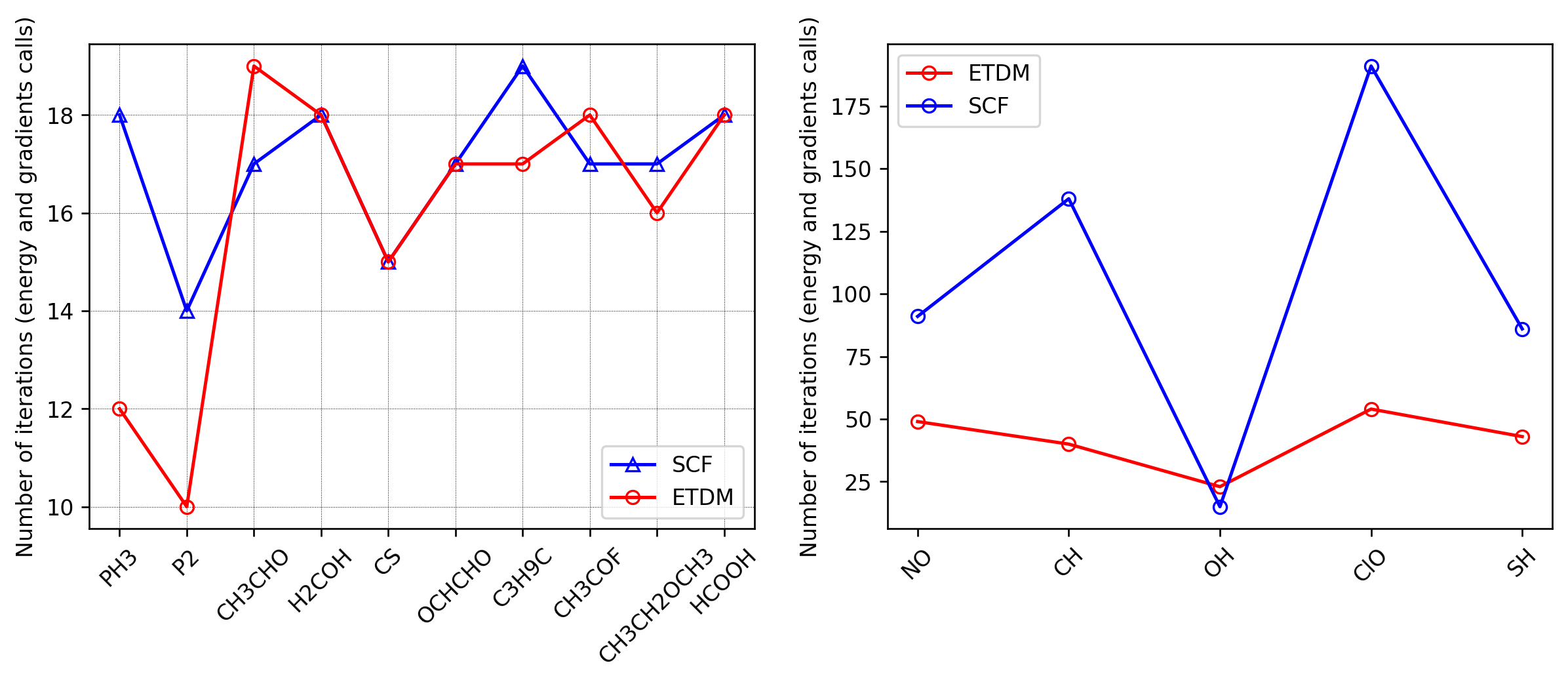
Here we compare the number of energy and gradient evaluations in direct minimization using the L-BFGS algorithm (memory=3) with preconditioning and the number of iterations in the SCF LCAO eigensolver with default density mixing. The left panel of the figure below shows several examples for molecules from the G2 set. The right panel shows the results of direct minimization and SCF for molecules that are difficult to converge; these molecules are radicals and the calculations are carried out within spin-polarized DFT. Direct minimization demonstrates stable performance in all cases. Note that by choosing different parameters for the density mixing one may improve the convergence of the SCF methods.

The calculations were run with the script g2_dm_ui_vs_scf.py, while the figure was generated using plot_g2.py.

32-128 Water Molecules

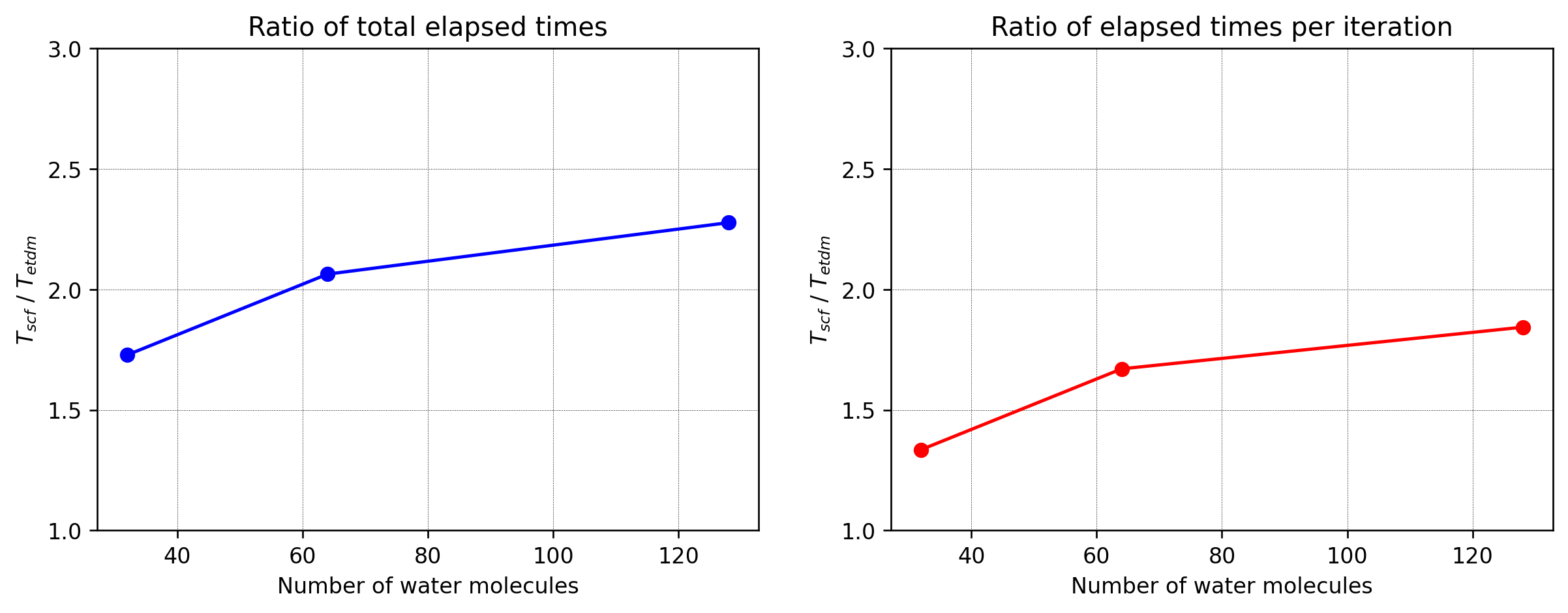
In this test, the ground state of liquid water configurations with 32, 64, 128 molecules and the TZDP basis set is calculated. The geometries are taken from here. The GPAW parameters used in this test include: PBE functional, grid spacing h=0.2 Å, and 8-core domain decomposition. The convergence criterion is a change in density smaller than \(10^{-6}\) electrons per valence electron. The ratio of the elapsed times spent by the default LCAO eigensolver and the direct minimization methods as a function of the number of water molecules is shown below. In direct minimization, the unitary invariant representation has been used [4] (see Implementation Details). As can be seen, direct minimization converges faster by around a factor of 1.5 for 32 molecules and around a factor of 2 for 128 molecules.

The calculations were run with the script wm_dm_vs_scf.py, while the figure was generated using plot_h2o.py.

Implementation Details

The implementation follows ref. [2] The iteratives are:

\[A^{(k+1)} = A^{(k)} + \gamma^{(k)} Q^{(k)}\]

where \(Q\) is the search direction and \(\gamma\) is step length. The search direction is calculated according to the L-BFGS algorithm with preconditioning, and the step length satisfies the Strong Wolfe Conditions [5] and/or approximate Wolfe Conditions [6]. The last two conditions are important as they guarantee stability and fast convergence of the L-BFGS algorithm [5]. Apart from the L-BFGS algorithm, one can use a limited-memory symmetric rank-one (L-SR1, default memory 20) quasi-Newton algorithm, which has also been shown to have good convergence performance and is especially recommended for calculations of excited states [3] (see also Excited-State Calculations with Maximum Overlap Method and Direct Optimization ). There is also an option to use a conjugate gradient algorithm, but it is less efficient.

Here are the three algorithms that can be used to calculate the matrix exponential:

1. The scaling and squaring algorithm, which is based on the equation:

   \[\exp(A) = \exp(A/2^{m})^{2^{m}}\]

   Since \(A/2^{m}\) has a small norm, then \(\exp(A/2^{m})\) can be effectively estimated using a Pade approximant of order \([q/q]\). Here q and m are positive integers. The scaling and squaring algorithm algorithm of Al-Moly and Higham [7] from the SciPy library is used.

2. Using the eigendecompostion of the matrix \(iA\). Let \(\Omega\) be a diagonal real-valued matrix with elements corresponding to the eigenvalues of the matrix \(iA\), and let \(U\) be the matrix having as columns the eigenvectors of \(iA\). Then the matrix exponential of \(A\) is:

   \[\exp(A) = U \exp(-i\Omega) U^{\dagger}\]

3. For a unitary invariant functional, the matrix \(A\) can be parametrized as [4]:

   \[\begin{split}A = \begin{pmatrix} 0 & A_{ov} \\ -A_{ov}^{\dagger} & 0 \end{pmatrix}\end{split}\]

   where \(A_{ov}\) is a \(N \times (M-N)\) matrix, where \(N\) is the number of occupied states and \(M\) is the number of basis functions, while \(0\) is an \(N \times N\) zero matrix. In this case the matrix exponential can be calculated as [4]:

   \[\begin{split}\exp(A) = \begin{pmatrix} \cos(P) & P^{-1/2} \sin(P^{1/2}) A_{ov}\\ -A_{ov}^{\dagger} P^{-1/2} \sin(P^{1/2}) & I_{M-N} + A_{ov}^{\dagger}\cos(P^{1/2} - I_N) P^{-1} A_{ov} ) \end{pmatrix}\end{split}\]

   where \(P = A_{ov}A_{ov}^{\dagger}\)

The first method is the default choice. To use the second algorithm do the following:

from gpaw.directmin.etdm_lcao import LCAOETDM
calc = GPAW(eigensolver=LCAOETDM(matrix_exp='egdecomp'),
            ...)

To use the third method, first ensure that your functional is unitary invariant and then do the following:

from gpaw.directmin.etdm_lcao import LCAOETDM
calc = GPAW(eigensolver=LCAOETDM(matrix_exp='egdecomp-u-invar',
                                 representation='u-invar'),
            ...)

The last option is the most efficient but it is valid only for a unitary invariant functionals (e.g. when all occupied orbitals of a given spin channel have the same occupation number)

For all three algorithms, the unitary invariant representation can be chosen.

ScaLAPCK and the parallelization over bands are currently not supported. It is also not recommended to use the direct minimization for metals because the occupation numbers are not found variationally but rather fixed during the calculation.

References

[1]

A. V. Ivanov, G. Levi, E.Ö. Jónsson, and H. Jónsson, J. Chem. Theory Comput., 17, 5034, (2021).

[2]

A. V. Ivanov, E.Ö. Jónsson, T. Vegge, and H. Jónsson, Comput. Phys. Commun., 267, 108047 (2021).

[3]

G. Levi, A. V. Ivanov, and H. Jónsson, J. Chem. Theory Comput., 16, 6968, (2020).

[4] (1,2,3)

J. Hutter, M. Parrinello, and S. Vogel, J. Chem. Phys. 101, 3862 (1994)

[5] (1,2)

J. Nocedal and S. J. Wright, Numerical Optimization, 2nd ed. (Springer, New York, NY, USA, 2006).

[6]

W. W. Hager and H. Zhang, SIAM Journal on Optimization 16, 170 (2006).

[7]

A. H. Al-Moly, and N. J. Higham, SIAM J. Matrix Anal. Appl., 31(3), 970–989, (2009).