Hybrid Quantum/Classical Scheme
The basic idea is to separate the calculation into two parts: the first one is the quantum subsystem, which is propagated using Time-propagation TDDFT scheme, and the second one is the classical subsystem that is treated using Quasistatic Finite-Difference Time-Domain method. The subsystems are propagated separately in their own real space grids, but they share a common electrostatic potential.
In the Time-propagation TDDFT part of the calculation the electrostatic potential is known as the Hartree potential \(V^{\rm{qm}}(\mathbf{r}, t)\) and it is solved from the Poisson equation \(\nabla^2 V^{\rm{qm}}(\mathbf{r}, t) = -4\pi\rho^{\rm{qm}}(\mathbf{r}, t)\)
In the Quasistatic Finite-Difference Time-Domain method the electrostatic potential is solved from the Poisson equation as well: \(V^{\rm{cl}}(\mathbf{r}, t) = -4\pi\rho^{\rm{cl}}(\mathbf{r}, t).\)
The hybrid scheme is created by replacing in both schemes the electrostatic (Hartree) potential by a common potential: \(\nabla^2 V^{\rm{tot}}(\mathbf{r}, t) = -4\pi\left[\rho^{\rm{cl}}(\mathbf{r}, t)+\rho^{\rm{qm}}(\mathbf{r}, t)\right].\)
Double grid
The observables of the quantum and classical subsystems are defined in their own grids, which are overlapping but can have different spacings. The following restrictions must hold:
The quantum grid must fit completely inside the classical grid
The spacing of the classical grid \(h_{\rm{cl}}\) must be equal to \(2^n h_{\rm{qm}}\), where \(h_{\rm{qm}}\) is the spacing of the quantum grid and n is an integer.
When these conditions hold, the potential from one subsystem can be transferred to the other one. The grids are automatically adjusted so that some grid points are common.
Transferring the potential between two grids
Transferring the potential from classical subsystem to the quantum grid is performed by interpolating the classical potential to the denser grid of the quantum subsystem. The interpolation only takes place in the small subgrid around the quantum mechanical region.
Transferring the potential from quantum subsystem to the classical one is done in another way: instead of the potential itself, it is the quantum mechanical electron density \(\rho^{\rm{qm}}(\mathbf{r}, t)\) that is copied to the coarser classical grid. Its contribution to the total electrostatic potential is then determined by solving the Poisson equation in that grid.
Altogether this means that although there is only one potential to be determined \((V^{\rm{tot}}(\mathbf{r}, t))\), three Poisson equations must be solved:
\(V^{\rm{cl}}(\mathbf{r}, t)\) in classical grid
\(V^{\rm{qm}}(\mathbf{r}, t)\) in quantum grid
\(V^{\rm{qm}}(\mathbf{r}, t)\) in classical grid
When these are ready and \(V^{\rm{cl}}(\mathbf{r}, t)\) is transferred to the quantum grid, \(V^{\rm{tot}}(\mathbf{r}, t)\) is determined in both grids.
Example: photoabsorption of Na2 near gold nanosphere
This example calculates the photoabsorption of \(\text{Na}_2\) molecule in (i) presence and (ii) absence of a gold nanosphere:
from ase import Atoms
from gpaw.fdtd.poisson_fdtd import QSFDTD
from gpaw.fdtd.polarizable_material import (PermittivityPlus,
                                            PolarizableMaterial,
                                            PolarizableSphere)
from gpaw.tddft import photoabsorption_spectrum
import numpy as np

# Nanosphere radius (Angstroms)
radius = 7.40

# Geometry
atom_center = np.array([30., 15., 15.])
sphere_center = np.array([15., 15., 15.])
simulation_cell = np.array([40., 30., 30.])

# Atoms object
atoms = Atoms('Na2', atom_center + np.array([[-1.5, 0.0, 0.0],
                                             [1.5, 0.0, 0.0]]))

# Permittivity of Gold
# J. Chem. Phys. 135, 084121 (2011); https://dx.doi.org/10.1063/1.3626549
eps_gold = PermittivityPlus(data=[[0.2350, 0.1551, 95.62],
                                  [0.4411, 0.1480, -12.55],
                                  [0.7603, 1.946, -40.89],
                                  [1.161, 1.396, 17.22],
                                  [2.946, 1.183, 15.76],
                                  [4.161, 1.964, 36.63],
                                  [5.747, 1.958, 22.55],
                                  [7.912, 1.361, 81.04]])

# 1) Nanosphere only
classical_material = PolarizableMaterial()
classical_material.add_component(PolarizableSphere(center=sphere_center,
                                                   radius=radius,
                                                   permittivity=eps_gold))

qsfdtd = QSFDTD(classical_material=classical_material,
                atoms=None,
                cells=simulation_cell,
                spacings=[2.0, 0.5],
                remove_moments=(1, 1))

energy = qsfdtd.ground_state('gs.gpw', mode='fd', nbands=1, symmetry='off')

qsfdtd.time_propagation('gs.gpw',
                        kick_strength=[0.001, 0.000, 0.000],
                        time_step=10,
                        iterations=1500,
                        dipole_moment_file='dm.dat')

photoabsorption_spectrum('dm.dat', 'spec.1.dat', width=0.15)


# 2) Na2 only (radius=0)
classical_material = PolarizableMaterial()
classical_material.add_component(PolarizableSphere(center=sphere_center,
                                                   radius=0.0,
                                                   permittivity=eps_gold))

qsfdtd = QSFDTD(classical_material=classical_material,
                atoms=atoms,
                cells=(simulation_cell, 4.0),  # vacuum = 4.0 Ang
                spacings=[2.0, 0.5],
                remove_moments=(1, 1))

energy = qsfdtd.ground_state('gs.gpw', mode='fd', nbands=-1, symmetry='off')

qsfdtd.time_propagation('gs.gpw',
                        kick_strength=[0.001, 0.000, 0.000],
                        time_step=10,
                        iterations=1500,
                        dipole_moment_file='dm.dat')

photoabsorption_spectrum('dm.dat', 'spec.2.dat', width=0.15)

# 3) Nanosphere + Na2
classical_material = PolarizableMaterial()
classical_material.add_component(PolarizableSphere(center=sphere_center,
                                                   radius=radius,
                                                   permittivity=eps_gold))

qsfdtd = QSFDTD(classical_material=classical_material,
                atoms=atoms,
                cells=(simulation_cell, 4.0),  # vacuum = 4.0 Ang
                spacings=[2.0, 0.5],
                remove_moments=(1, 1))

energy = qsfdtd.ground_state('gs.gpw', mode='fd', nbands=-1, symmetry='off')

qsfdtd.time_propagation('gs.gpw',
                        kick_strength=[0.001, 0.000, 0.000],
                        time_step=10,
                        iterations=1500,
                        dipole_moment_file='dm.dat')

photoabsorption_spectrum('dm.dat', 'spec.3.dat', width=0.15)
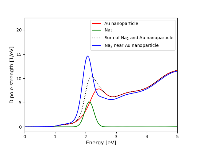
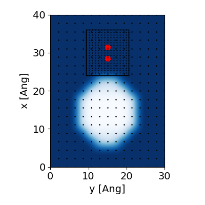
The optical response of the molecule apparently enhances when
it is located near the metallic nanoparticle, see Ref. [1] for
more examples. The geometry and the distribution
of the grid points are shown in the following figure
(generated with this script):
Advanced example: Near field enhancement of hybrid system
In this example we calculate the same hybrid Na2 + gold nanoparticle
system as above, but using the advanced syntax instead of the
QSFDTD wrapper. This allows us to include InducedField observers
in the calculation, see
TDDFTInducedField module documentation:
from ase import Atoms
from gpaw import GPAW
from gpaw.fdtd.poisson_fdtd import FDTDPoissonSolver
from gpaw.fdtd.polarizable_material import (PermittivityPlus,
                                            PolarizableMaterial,
                                            PolarizableSphere)
from gpaw.tddft import TDDFT, DipoleMomentWriter, photoabsorption_spectrum
from gpaw.inducedfield.inducedfield_tddft import TDDFTInducedField
from gpaw.inducedfield.inducedfield_fdtd import FDTDInducedField
from gpaw.mpi import world
import numpy as np

# Nanosphere radius (Angstroms)
radius = 7.40

# Geometry
atom_center = np.array([30., 15., 15.])
sphere_center = np.array([15., 15., 15.])
simulation_cell = np.array([40., 30., 30.])

# Atoms object
atoms = Atoms('Na2', atom_center + np.array([[-1.5, 0.0, 0.0],
                                             [1.5, 0.0, 0.0]]))

# Permittivity of Gold
# J. Chem. Phys. 135, 084121 (2011); https://dx.doi.org/10.1063/1.3626549
eps_gold = PermittivityPlus(data=[[0.2350, 0.1551, 95.62],
                                  [0.4411, 0.1480, -12.55],
                                  [0.7603, 1.946, -40.89],
                                  [1.161, 1.396, 17.22],
                                  [2.946, 1.183, 15.76],
                                  [4.161, 1.964, 36.63],
                                  [5.747, 1.958, 22.55],
                                  [7.912, 1.361, 81.04]])

# 3) Nanosphere + Na2
classical_material = PolarizableMaterial()
classical_material.add_component(PolarizableSphere(center=sphere_center,
                                                   radius=radius,
                                                   permittivity=eps_gold))

# Combined Poisson solver
poissonsolver = FDTDPoissonSolver(classical_material=classical_material,
                                  qm_spacing=0.5,
                                  cl_spacing=2.0,
                                  cell=simulation_cell,
                                  communicator=world,
                                  remove_moments=(1, 1))
poissonsolver.set_calculation_mode('iterate')

# Combined system
atoms.set_cell(simulation_cell)
atoms, qm_spacing, gpts = poissonsolver.cut_cell(atoms, vacuum=4.0)

# Initialize GPAW
gs_calc = GPAW(mode='fd',
               gpts=gpts,
               nbands=-1,
               poissonsolver=poissonsolver,
               symmetry={'point_group': False})
atoms.calc = gs_calc

# Ground state
energy = atoms.get_potential_energy()

# Save state
gs_calc.write('gs.gpw', 'all')

# Initialize TDDFT and FDTD
kick = [0.001, 0.000, 0.000]
time_step = 10
iterations = 1500

td_calc = TDDFT('gs.gpw')
DipoleMomentWriter(td_calc, 'dm.dat')

# Attach InducedFields to the calculation
frequencies = [2.05, 2.60]
width = 0.15
cl_ind = FDTDInducedField(paw=td_calc,
                          frequencies=frequencies,
                          width=width)
qm_ind = TDDFTInducedField(paw=td_calc,
                           frequencies=frequencies,
                           width=width)

# Propagate TDDFT and FDTD
td_calc.absorption_kick(kick_strength=kick)
td_calc.propagate(time_step, iterations)

# Save results
td_calc.write('td.gpw', 'all')
cl_ind.write('cl.ind')
qm_ind.write('qm.ind')

photoabsorption_spectrum('dm.dat', 'spec.3.dat', width=width)
The TDDFTInducedField records the quantum part of the calculation and
the FDTDInducedField records the classical part.
We can calculate the individual and the total induced field
by the following script:
from gpaw.tddft import TDDFT
from gpaw.inducedfield.inducedfield_fdtd import (
    FDTDInducedField, calculate_hybrid_induced_field)
from gpaw.inducedfield.inducedfield_tddft import TDDFTInducedField

td_calc = TDDFT('td.gpw')

# Classical subsystem
cl_ind = FDTDInducedField(filename='cl.ind', paw=td_calc)
cl_ind.calculate_induced_field(gridrefinement=2)
cl_ind.write('cl_field.ind', mode='all')

# Quantum subsystem
qm_ind = TDDFTInducedField(filename='qm.ind', paw=td_calc)
qm_ind.calculate_induced_field(gridrefinement=2)
qm_ind.write('qm_field.ind', mode='all')

# Total system, interpolate/extrapolate to a grid with spacing h
tot_ind = calculate_hybrid_induced_field(cl_ind, qm_ind, h=1.0)
tot_ind.write('tot_field.ind', mode='all')
All the InducedField objects
can be analyzed in the same way as described in
TDDFTInducedField module documentation.
Here we show an example script
for plotting (run in serial mode, i.e., with one process):
# web-page: cl_field.ind_Ffe.png, qm_field.ind_Ffe.png, tot_field.ind_Ffe.png
from gpaw.mpi import world
import numpy as np
import matplotlib.pyplot as plt
from gpaw.inducedfield.inducedfield_base import BaseInducedField
from gpaw.tddft.units import aufrequency_to_eV
assert world.size == 1, 'This script should be run in serial mode.'
# Helper function
def do_plot(d_g, ng, box, atoms):
# Take slice of data array
d_yx = d_g[:, :, ng[2] // 2]
y = np.linspace(0, box[0], ng[0] + 1)[:-1]
dy = box[0] / (ng[0] + 1)
y += dy * 0.5
ylabel = u'x / Å'
x = np.linspace(0, box[1], ng[1] + 1)[:-1]
dx = box[1] / (ng[1] + 1)
x += dx * 0.5
xlabel = u'y / Å'
# Plot
plt.figure()
ax = plt.subplot(1, 1, 1)
X, Y = np.meshgrid(x, y)
plt.contourf(X, Y, d_yx, 40)
plt.colorbar()
for atom in atoms:
pos = atom.position
plt.scatter(pos[1], pos[0], s=50, c='k', marker='o')
plt.xlabel(xlabel)
plt.ylabel(ylabel)
plt.xlim([x[0], x[-1]])
plt.ylim([y[0], y[-1]])
ax.set_aspect('equal')
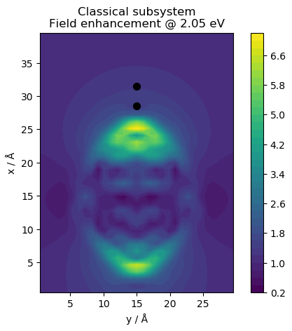
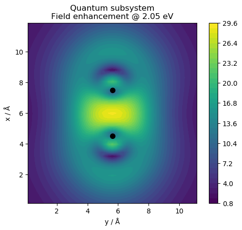
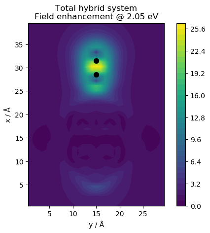
for fname, name in zip(['cl_field.ind', 'qm_field.ind', 'tot_field.ind'],
['Classical subsystem', 'Quantum subsystem',
'Total hybrid system']):
# Read InducedField object
ind = BaseInducedField(fname, readmode='all')
# Choose array
w = 0 # Frequency index
freq = ind.omega_w[w] * aufrequency_to_eV # Frequency
box = np.diag(ind.atoms.get_cell()) # Calculation box
d_g = ind.Ffe_wg[w] # Data array
ng = d_g.shape # Size of grid
atoms = ind.atoms # Atoms
do_plot(d_g, ng, box, atoms)
plt.title(f'{name}\nField enhancement @ {freq:.2f} eV')
plt.savefig(fname + '_Ffe.png', bbox_inches='tight')
# Imaginary part of density
d_g = ind.Frho_wg[w].imag
ng = d_g.shape
do_plot(d_g, ng, box, atoms)
plt.title('%s\nImaginary part of induced charge density @ %.2f eV' %
(name, freq))
plt.savefig(fname + '_Frho.png', bbox_inches='tight')
# Imaginary part of potential
d_g = ind.Fphi_wg[w].imag
ng = d_g.shape
do_plot(d_g, ng, box, atoms)
plt.title(f'{name}\nImaginary part of induced potential @ {freq:.2f} eV')
plt.savefig(fname + '_Fphi.png', bbox_inches='tight')
This produces the following figures for the electric near field: