Spin-orbit coupling and non-collinear calculations
https://journals.aps.org/prb/abstract/10.1103/PhysRevB.62.11556
from gpaw.new.ase_interface import GPAW
from ase import Atoms
import numpy as np

a = 6.339
d = 1.331

atoms = Atoms('V3Cl6',
              cell=[a, a, 1, 90, 90, 60],
              pbc=[1, 1, 0],
              scaled_positions=[
                  [0, 0, 0],
                  [1 / 3, 1 / 3, 0],
                  [2 / 3, 2 / 3, 0],
                  [0, 2 / 3, d],
                  [0, 1 / 3, -d],
                  [1 / 3, 0, d],
                  [1 / 3, 2 / 3, -d],
                  [2 / 3, 1 / 3, d],
                  [2 / 3, 0, -d]])
atoms.center(axis=2, vacuum=5)

m = 3.0
magmoms = np.zeros((9, 3))
magmoms[0] = [m, 0, 0]
magmoms[1] = [-m / 2, m * 3**0.5 / 2, 0]
magmoms[2] = [-m / 2, -m * 3**0.5 / 2, 0]

atoms.calc = GPAW(mode={'name': 'pw',
                        'ecut': 400},
                  magmoms=magmoms,
                  symmetry='off',
                  kpts={'size': (2, 2, 1), 'gamma': True},
                  parallel={'domain': 1, 'band': 1},
                  txt='VCl2_gs.txt')

atoms.get_potential_energy()
atoms.calc.write('VCl2_gs.gpw')
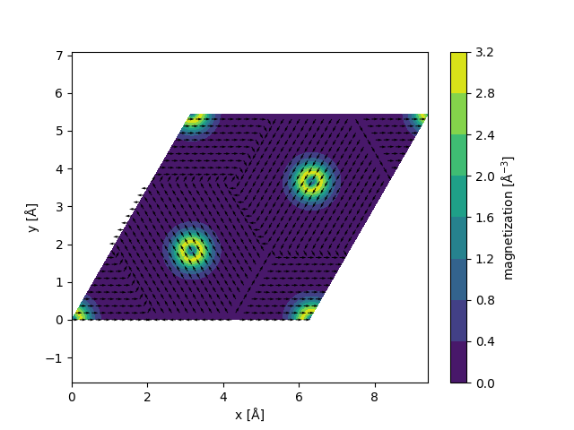
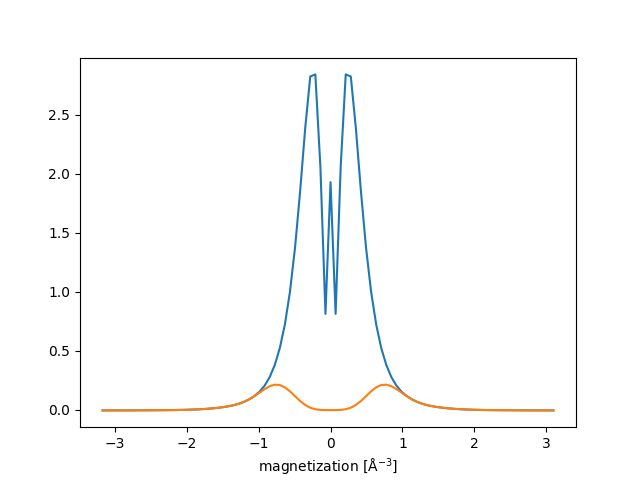
# web-page: mag1d.png, mag2d.png
from gpaw.new.ase_interface import GPAW
import matplotlib.pyplot as plt
import numpy as np

calc = GPAW('VCl2_gs.gpw')
dens = calc.dft.densities()
grid_spacing = calc.atoms.cell[2, 2] / 200
nt = dens.pseudo_densities(grid_spacing)
n = dens.all_electron_densities(grid_spacing=grid_spacing)

i = nt.desc.size[2] // 2
x, y = n.desc.xyz()[:, :, i, :2].transpose((2, 0, 1))
uv = n.data[1:3, :, :, i]
m = (uv**2).sum(0)**0.5
u, v = uv / m
fig, ax = plt.subplots()
ct = ax.contourf(x, y, m)
cbar = fig.colorbar(ct)
cbar.ax.set_ylabel('magnetization [Å$^{-3}$]')
ax.quiver(*(a[::3, ::3] for a in [x, y, u, v]))
ax.axis('equal')
ax.set_xlabel('x [Å]')
ax.set_ylabel('y [Å]')
fig.savefig('mag2d.png')

fig, ax = plt.subplots()
x, y = n.xy(1, ..., 0, i)
x, yt = nt.xy(1, ..., 0, i)
j = len(x) // 2
L = calc.atoms.cell[0, 0]
x = np.concatenate((x[j:] - L, x[:j]))
y = np.concatenate((y[j:], y[:j]))
yt = np.concatenate((yt[j:], yt[:j]))
ax.plot(x, y, label='all-electron')
ax.plot(x, yt, label='pseudo')
ax.legend()
ax.set_xlabel('x [Å]')
ax.set_ylabel('magnetization [Å$^{-3}$]')
fig.savefig('mag1d.png')
Experiential:
Theoretical:
DFT: