Quasistatic Finite-Difference Time-Domain method
The optical properties of all materials depend on how they respond (absorb and scatter) to external electromagnetic fields. In classical electrodynamics, this response is described by the Maxwell equations. One widely used method for solving them numerically is the finite-difference time-domain (FDTD) approach. [1]. It is based on propagating the electric and magnetic fields in time under the influence of an external perturbation (light) in such a way that the observables are expressed in real space grid points. The optical constants are obtained by analyzing the resulting far-field pattern. In the microscopic limit of classical electrodynamics the quasistatic approximation is valid and an alternative set of time-dependent equations for the polarization charge, polarization current, and the electric field can be derived.[2]
The quasistatic formulation of FDTD is implemented in GPAW. It can be used to model the optical properties of metallic nanostructures (i) purely classically, or (ii) in combination with Time-propagation TDDFT, which yields Hybrid Quantum/Classical Scheme.
Quasistatic approximation
The quasistatic approximation of classical electrodynamics means that the retardation effects due to the finite speed of light are neglected. It is valid at very small length scales, typically below ~50 nm.
Compared to full FDTD, quasistatic formulation has some advantageous features. The magnetic field is negligible and only the longitudinal electric field need to be considered, so the number of degrees of freedom is smaller. Because the retardation effects and propagating solutions are excluded, longer time steps and a simpler treatment of the boundary conditions can be used.
Permittivity
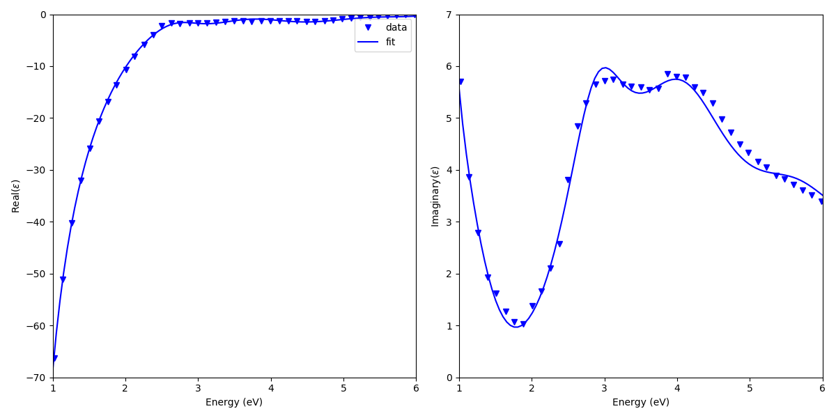
In the current implementation, the permittivity of the classical material is parametrized as a linear combination of Lorentzian oscillators
where \(\alpha_j, \beta_j, \bar{\omega}_j\) are fitted to reproduce the experimental permittivity. For gold and silver they can be found in Ref. [2]. Permittivity defines how classical charge density polarizes when it is subject to external electric fields. The time-evolution for the charges in GPAW is performed with the leap-frog algorithm, following Ref. [3].
To test the quality of the fit, one can use
this script.
This gives a following plot for Au permittivity fitting.
Geometry components
Several routines are available to generate the basic shapes:
\(\text{PolarizableBox}(\mathbf{r}_1, \mathbf{r}_2, \epsilon({\mathbf{r}, \omega}))\) where \(\mathbf{r}_1\) and \(\mathbf{r}_2\) are the corner points, and \(\epsilon({\mathbf{r}, \omega})\) is the permittivity inside the structure
\(\text{PolarizableSphere}(\mathbf{p}, r, \epsilon({\mathbf{r}, \omega}))\) where \(\mathbf{p}\) is the center and \(r\) is the radius of the sphere
\(\text{PolarizableEllipsoid}(\mathbf{p}, \mathbf{r}, \epsilon({\mathbf{r}, \omega}))\) where \(\mathbf{p}\) is the center and \(\mathbf{r}\) is the array containing the three radii
\(\text{PolarizableRod}(\mathbf{p}, r, \epsilon({\mathbf{r}, \omega}), c)\) where \(\mathbf{p}\) is an array of subsequent corner coordinates, \(r\) is the radius, and \(c\) is a boolean denoting whether the corners are rounded
\(\text{PolarizableTetrahedron}(\mathbf{p}, \epsilon({\mathbf{r}, \omega}))\) where \(\mathbf{p}\) is an array containing the four corner points of the tetrahedron
These routines can generate many typical geometries, and for general cases a set of tetrahedra can be used.
Optical response
The QSFDTD method can be used to calculate the optical photoabsorption spectrum just like in Time-propagation TDDFT: The classical charge density is first perturbed with an instantaneous electric field, and then the time dependence of the induced dipole moment is recorderd. Its Fourier transformation gives the photoabsorption spectrum.
Example: photoabsorption of gold nanosphere
This example calculates the photoabsorption spectrum of a nanosphere that has a diameter of 10 nm, and compares the result with analytical Mie scattering limit.
from gpaw.fdtd.poisson_fdtd import QSFDTD
from gpaw.fdtd.polarizable_material import (PermittivityPlus,
                                            PolarizableMaterial,
                                            PolarizableSphere)
from gpaw.tddft import photoabsorption_spectrum
from gpaw.mpi import world
import numpy as np

# Nanosphere radius (Angstroms)
radius = 50.0

# Whole simulation cell (Angstroms)
large_cell = np.array([3 * radius, 3 * radius, 3 * radius])

# Permittivity of Gold
# J. Chem. Phys. 135, 084121 (2011); https://dx.doi.org/10.1063/1.3626549
gold = [[0.2350, 0.1551, 95.62],
        [0.4411, 0.1480, -12.55],
        [0.7603, 1.946, -40.89],
        [1.161, 1.396, 17.22],
        [2.946, 1.183, 15.76],
        [4.161, 1.964, 36.63],
        [5.747, 1.958, 22.55],
        [7.912, 1.361, 81.04]]

# Initialize classical material
classical_material = PolarizableMaterial()

# Classical nanosphere
classical_material.add_component(
    PolarizableSphere(center=0.5 * large_cell,
                      radius=radius,
                      permittivity=PermittivityPlus(data=gold)))

# Quasistatic FDTD
qsfdtd = QSFDTD(classical_material=classical_material,
                atoms=None,
                cells=large_cell,
                spacings=[8.0, 1.0],
                communicator=world,
                remove_moments=(4, 1))

# Run ground state
energy = qsfdtd.ground_state('gs.gpw', mode='fd', nbands=-1, symmetry='off')

# Run time evolution
qsfdtd.time_propagation('gs.gpw',
                        time_step=10,
                        iterations=1000,
                        kick_strength=[0.001, 0.000, 0.000],
                        dipole_moment_file='dm.dat')
# Spectrum
photoabsorption_spectrum('dm.dat', 'spec.dat', width=0.0)
Here the QSFDTD object generates a dummy quantum system that is treated using GPAW in qsfdtd.ground_state. One can pass the GPAW arguments, like xc or nbands, to this function: in the example script one empty KS-orbital was included (nbands =1) because GPAW needs to propagate something. Similarly, the arguments for TDDFT (such as propagator) can be passed to time_propagation method.
Note that the permittivity was initialized as PermittivityPlus, where Plus indicates that a renormalizing Lorentzian term is included; this extra term brings the static limit to vacuum value, i.e., \(\epsilon(\omega=0)=\epsilon_0\), see Ref. [4] for detailed explanation.
The above script generates the photoabsorption spectrum and compares it with analytical formula of the Mie theory:
where V is the nanosphere volume:
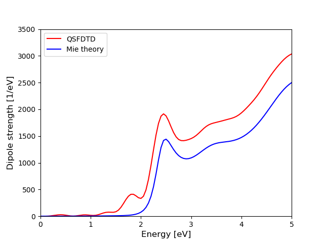
The general shape of Mie spectrum, and especially the localized surface plasmon resonance (LSPR) at 2.5 eV, is clearly reproduced by QSFDTD. The shoulder at 1.9 eV and the stronger overall intensity are examples of the inaccuracies of the used discretization scheme: the shoulder originates from spurious surface scattering, and the intensity from the larger volume of the nanosphere defined in the grid. For a better estimate of the effective volume, you can take a look at the standard output where the “Fill ratio” tells that 18.035% of the grid points locate inside the sphere. This means that the volume (and intensity) is roughly 16% too large:
\(\frac{V}{V_{\text{sphere}}}\approx\frac{0.18035\times(15\text{nm})^3)}{\frac{4}{3}\pi\times(5\text{nm})^3}\approx1.16\).
Advanced example: Near field enhancement
This example shows how to calculate the induced electric near field
enhancement of the same nanosphere considered in the previous example.
The induced field calculations can be included by using the advanced
syntax instead of the simple QSFDTD wrapper.
In the example one can also see how the dummy empty quantum system is
generated.
from ase import Atoms
from gpaw import GPAW
from gpaw.fdtd.poisson_fdtd import FDTDPoissonSolver
from gpaw.fdtd.polarizable_material import (PermittivityPlus,
                                            PolarizableMaterial,
                                            PolarizableSphere)
from gpaw.tddft import TDDFT, DipoleMomentWriter, photoabsorption_spectrum
from gpaw.inducedfield.inducedfield_fdtd import FDTDInducedField
from gpaw.mpi import world
import numpy as np

# Nanosphere radius (Angstroms)
radius = 50.0

# Whole simulation cell (Angstroms)
large_cell = np.array([3 * radius, 3 * radius, 3 * radius])

# Permittivity of Gold
# J. Chem. Phys. 135, 084121 (2011); https://dx.doi.org/10.1063/1.3626549
gold = [[0.2350, 0.1551, 95.62],
        [0.4411, 0.1480, -12.55],
        [0.7603, 1.946, -40.89],
        [1.161, 1.396, 17.22],
        [2.946, 1.183, 15.76],
        [4.161, 1.964, 36.63],
        [5.747, 1.958, 22.55],
        [7.912, 1.361, 81.04]]

# Initialize classical material
classical_material = PolarizableMaterial()

# Classical nanosphere
classical_material.add_component(
    PolarizableSphere(center=0.5 * large_cell,
                      radius=radius,
                      permittivity=PermittivityPlus(data=gold)))

# Poisson solver
poissonsolver = FDTDPoissonSolver(classical_material=classical_material,
                                  cl_spacing=8.0,
                                  qm_spacing=1.0,
                                  cell=large_cell,
                                  communicator=world,
                                  remove_moments=(4, 1))
poissonsolver.set_calculation_mode('iterate')

# Dummy quantum system
atoms = Atoms('H', [0.5 * large_cell], cell=large_cell)
atoms, qm_spacing, gpts = poissonsolver.cut_cell(atoms)
del atoms[:]  # Remove atoms, quantum system is empty

# Initialize GPAW
gs_calc = GPAW(mode='fd',
               gpts=gpts,
               nbands=-1,
               poissonsolver=poissonsolver,
               symmetry={'point_group': False})
atoms.calc = gs_calc

# Ground state
energy = atoms.get_potential_energy()

# Save state
gs_calc.write('gs.gpw', 'all')

# Initialize TDDFT and FDTD
kick = [0.001, 0.000, 0.000]
time_step = 10
iterations = 1000

td_calc = TDDFT('gs.gpw')
DipoleMomentWriter(td_calc, 'dm0.dat')

# Attach InducedField to the calculation
frequencies = [2.45]
width = 0.0
ind = FDTDInducedField(paw=td_calc,
                       frequencies=frequencies,
                       width=width)

# Propagate TDDFT and FDTD
td_calc.absorption_kick(kick_strength=kick)
td_calc.propagate(time_step, iterations)

# Save results
td_calc.write('td.gpw', 'all')
ind.write('td.ind')

# Spectrum
photoabsorption_spectrum('dm0.dat', 'spec.dat', width=width)

# Induced field
ind.calculate_induced_field(gridrefinement=2)
ind.write('field.ind', mode='all')
The contents of the obtained file field.ind
can be visualized like described in
Advanced example: Near field enhancement of hybrid system.
We obtain a following plot of the field:
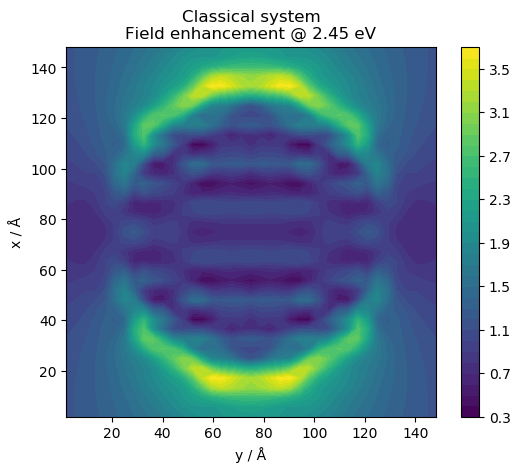
Note that the oscillations in the induced field (and density) inside the material are caused by numerical limitations of the current implementation.
Limitations
The scattering from the spurious surfaces of materials, which are present because of the representation of the polarizable material in uniformly spaced grid points, can cause unphysical broadening of the spectrum.
Nonlinear response (hyperpolarizability) of the classical material is not supported, so do not use too large external fields. In addition to nonlinear media, also other special cases (nonlocal permittivity, natural birefringence, dichroism, etc.) are not enabled.
The frequency-dependent permittivity of the classical material must be represented as a linear combination of Lorentzian oscillators. Other forms, such as Drude terms, should be implemented in the future. Also, the high-frequency limit must be vacuum permittivity. Future implementations should get rid of also this limitation.
Only the grid-mode of GPAW (not e.g. LCAO) is supported.
Technical remarks
Double grid technique: the calculation always uses two grids: one for the classical part and one for the TDDFT part. In purely classical simulations, suchs as the ones discussed in this page, the quantum subsystem contains one empty Kohn-Sham orbital. For more information, see the description of Hybrid Quantum/Classical Scheme because there the double grid is very important.
Parallelizatility: QSFDTD calculations can by parallelized only over domains, so use either communicator=serial_comm or communicator=world when initializing QSFDTD (or FDTDPoissonSolver) class. The domain parallelization of QSFDTD does not affect the parallelization of DFT calculation.
Multipole corrections to Poissonsolver: QSFDTD module is mainly intended for nanoplasmonic simulations. There the charge oscillations are strong and the usual zero boundary conditions for the electrostatic potential can give inaccurate results if the simulation box is not large enough. In some cases, such as for single nanospheres, one can improve the situation by defining remove_moments argument in FDTDPoissonSolver: this will then use the multipole moments correction scheme, see e.g. Ref. [5].
TODO
Dielectrics (\(\epsilon_{\infty}\neq\epsilon_0\))
Geometries from 3D model files
Sub-cell averaging
Full FDTD (retardation effects) or interface to an external FDTD software
Fix grid-dependent oscillations in the induced density
Combination with TDDFT
The QSFDTD module is mainly aimed to be used in combination with Time-propagation TDDFT: see Hybrid Quantum/Classical Scheme for more information.