Muon Site

Positive muons implanted in metals tend to stop at interstitial sites that correspond to the maxima of the Coulomb potential energy for electrons in the material. In turns the Coulomb potential is approximated by the Hartree pseudo-potential obtained from the GPAW calculation. A good guess is therefore given by the maxima of this potential.

In this tutorial we obtain the guess in the case of MnSi. The results can be compared with A. Amato et al. [Amato14], who find a muon site at fractional cell coordinates (0.532,0.532,0.532) by DFT calculations and by the analysis of experiments.

MnSi calculation

Let’s perform the calculation in ASE, starting from the space group of MnSi, 198, and the known Mn and Si coordinates.

from gpaw import GPAW, PW, MethfesselPaxton
from ase.spacegroup import crystal
from ase.io import write

a = 4.55643
mnsi = crystal(['Mn', 'Si'],
               [(0.1380, 0.1380, 0.1380), (0.84620, 0.84620, 0.84620)],
               spacegroup=198,
               cellpar=[a, a, a, 90, 90, 90])


for atom in mnsi:
    if atom.symbol == 'Mn':
        atom.magmom = 0.5

mnsi.calc = GPAW(xc='PBE',
                 kpts=(2, 2, 2),
                 mode=PW(800),
                 occupations=MethfesselPaxton(width=0.005),
                 txt='mnsi.txt')

mnsi.get_potential_energy()
mnsi.calc.write('mnsi.gpw')
v = mnsi.calc.get_electrostatic_potential()
write('mnsi.cube', mnsi, data=v)

The ASE code outputs a Gaussian cube file, mnsi.cube, with volumetric data of the potential (in eV) that can be visualized.

Getting the maximum

One way of identifying the maximum is by the use of an isosurface (or 3d contour surface) at a slightly lower value than the maximum. This can be done by means of an external visualization program, like eg. majavi (see also Plotting iso-surfaces with Mayavi):

$ python3 -m ase.visualize.mlab -c 11.1,13.3 mnsi.cube

The parameters after -c are the potential values for two countour surfaces (the maximum is 13.4 eV).

This allows also secondary (local) minima to be identified.

A simplified procedure to identify the global maximum is the following

# web-page: pot_contour.png
from gpaw import restart
import matplotlib.pyplot as plt
import numpy as np

mnsi, calc = restart('mnsi.gpw', txt=None)
v = calc.get_electrostatic_potential()
a = mnsi.cell[0, 0]
n = v.shape[0]
x = y = np.linspace(0, a, n, endpoint=False)

f = plt.figure()
ax = f.add_subplot(111)
cax = ax.contour(x, y, v[:, :, n // 2], 100)
cbar = f.colorbar(cax)
ax.set_xlabel('x (Angstrom)')
ax.set_ylabel('y (Angstrom)')
ax.set_title('Pseudo-electrostatic Potential')
f.savefig('pot_contour.png')

The figure below shows the contour plot of the pseudo-potential in the plane z=2.28 Ångström containing the maximum

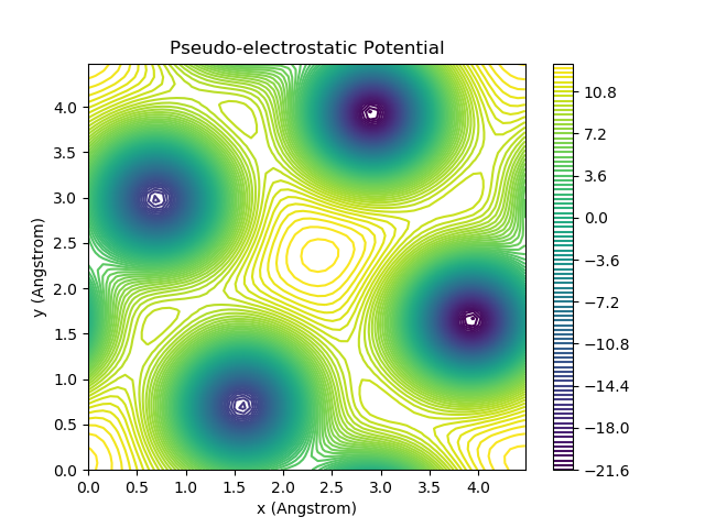
The absolute maximum is at the center of the plot, at (2.28,2.28,2.28), in Ångström. A local maximum is also visible around (0.6,1.75,2.28), in Ångström.

In comparing with [Amato14] keep in mind that the present examples has a reduced number of k points and a low plane wave cutoff energy, just enough to show the right extrema in the shortest CPU time.

---

[Amato14] (1,2)

A. Amato et al. Phys. Rev. B. 89, 184425 (2014) Understanding the μSR spectra of MnSi without magnetic polarons doi: 10.1103/PhysRevB.1.4555