Dipole-layer corrections in GPAW
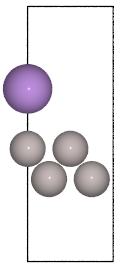
As an example system, a 2 layer \(2\times2\) slab of fcc (100) Al is constructed with a single Na adsorbed on one side of the surface.
from ase.build import fcc100, add_adsorbate
from gpaw import GPAW

slab = fcc100('Al', (2, 2, 2), a=4.05, vacuum=7.5)
add_adsorbate(slab, 'Na', 4.0)
slab.center(axis=2)

slab.calc = GPAW(mode='fd',
                 txt='zero.txt',
                 xc='PBE',
                 setups={'Na': '1'},
                 kpts=(4, 4, 1))
e1 = slab.get_potential_energy()
slab.calc.write('zero.gpw')
The ase.build.fcc100() function will create a slab
with periodic boundary conditions in the xy-plane only and GPAW will
therefore use zeros boundary conditions for the wave functions and
the electrostatic potential in the z-direction as shown here:
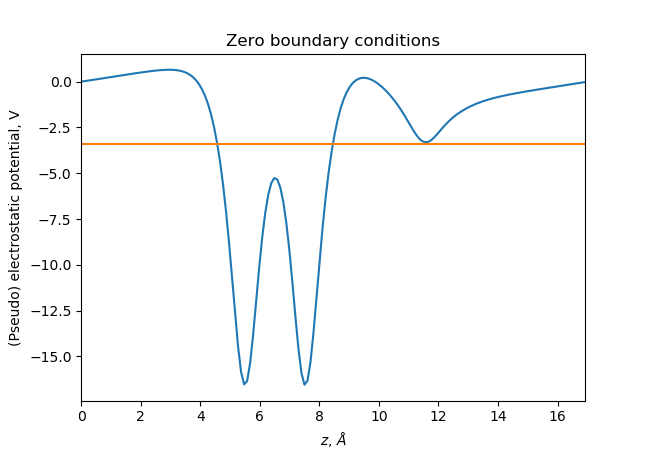
The blue line is the xy-averaged potential and the green line is the
fermi-level. See below how to extract the potential using the
get_electrostatic_potential() method.
If we use periodic boundary conditions in all directions:
slab.pbc = True
slab.calc = slab.calc.new(txt='periodic.txt')
e2 = slab.get_potential_energy()
the electrostatic potential will be periodic and average to zero:

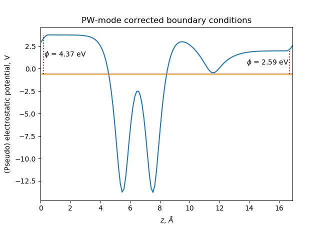
In order to estimate the work functions on the two sides of the slab, we need to have flat potentials or zero electric field in the vacuum region away from the slab. This can be achieved by using a dipole correction:
slab.pbc = (True, True, False)
slab.calc = slab.calc.new(poissonsolver={'dipolelayer': 'xy'},
                          txt='corrected.txt')
e3 = slab.get_potential_energy()

In PW-mode, the potential must be periodic and in that case the corrected potential looks like this (see [Bengtsson] for more details):
See the full Python scripts here dipole.py and here
pwdipole.py. The script
used to create the figures in this tutorial is shown here:
# web-page: zero.png, periodic.png, corrected.png, pwcorrected.png, slab.png
import numpy as np
import matplotlib.pyplot as plt
from ase.io import write
from gpaw import GPAW

# this test requires OpenEXR-libs

for name in ['zero', 'periodic', 'corrected', 'pwcorrected']:
    calc = GPAW(name + '.gpw', txt=None)

    efermi = calc.get_fermi_level()

    # Average over y and x:
    v = calc.get_electrostatic_potential().mean(1).mean(0)
    z = np.linspace(0, calc.atoms.cell[2, 2], len(v), endpoint=False)

    plt.figure(figsize=(6.5, 4.5))
    plt.plot(z, v, label='xy-averaged potential')
    plt.plot([0, z[-1]], [efermi, efermi], label='Fermi level')

    if name.endswith('corrected'):
        n = 6  # get the vacuum level 6 grid-points from the boundary
        plt.plot([0.2, 0.2], [efermi, v[n]], 'r:')
        plt.text(0.23, (efermi + v[n]) / 2,
                 r'$\phi$ = %.2f eV' % (v[n] - efermi), va='center')
        plt.plot([z[-1] - 0.2, z[-1] - 0.2], [efermi, v[-n]], 'r:')
        plt.text(z[-1] - 0.23, (efermi + v[-n]) / 2,
                 r'$\phi$ = %.2f eV' % (v[-n] - efermi),
                 va='center', ha='right')

    plt.xlabel(r'$z$, r$\AA$')
    plt.ylabel('(Pseudo) electrostatic potential, V')
    plt.xlim([0., z[-1]])
    if name == 'pwcorrected':
        title = 'PW-mode corrected'
    else:
        title = name.title()
    plt.title(title + ' boundary conditions')
    plt.savefig(name + '.png')

write('slab.pov',
      calc.atoms,
      rotation='-90x',
      show_unit_cell=2,
      povray_settings=dict(
          transparent=False,
          display=False)).render()
Lennart Bengtsson, Dipole correction for surface supercell calculations, Phys. Rev. B 59, 12301 - Published 15 May 1999