Jellium
In this tutorial, we try to reproduce some old jellium calculations by Lang and Kohn [Lang70].
Bulk
Let’s do a calculation for \(r_s=5\) Bohr. We use a cubic cell with a lattice constant of \(a=1.6\) Å, 8*8*8 grid points and and a k-point sampling of 12*12*12 points.
import numpy as np
from ase import Atoms
from ase.units import Bohr
from gpaw.jellium import Jellium
from gpaw import GPAW, PW

rs = 5.0 * Bohr  # Wigner-Seitz radius
h = 0.2          # grid-spacing
a = 8 * h        # lattice constant
k = 12           # number of k-points (k*k*k)

ne = a**3 / (4 * np.pi / 3 * rs**3)
jellium = Jellium(ne)

bulk = Atoms(pbc=True, cell=(a, a, a))
bulk.calc = GPAW(mode=PW(400.0),
                 background_charge=jellium,
                 xc='LDA_X+LDA_C_WIGNER',
                 nbands=5,
                 kpts=[k, k, k],
                 h=h,
                 txt='bulk.txt')
e0 = bulk.get_potential_energy()
In the text output from the calculation, one can see that the cell contains 0.0527907 electrons.
Surfaces
Now, we will do a surface calculation. We put a slab of thickness 16.0 Å inside a box, periodically repeated in the x- and y-directions only, of size 1.6*1.6*25.6 Å and use 12*12 k-points to sample the surface BZ:
import numpy as np
from ase import Atoms
from ase.units import Bohr
from gpaw.jellium import JelliumSlab
from gpaw import GPAW, PW

rs = 5.0 * Bohr  # Wigner-Seitz radius
h = 0.2          # grid-spacing
a = 8 * h        # lattice constant
v = 3 * a        # vacuum
L = 10 * a       # thickness
k = 12           # number of k-points (k*k*1)

ne = a**2 * L / (4 * np.pi / 3 * rs**3)

eps = 0.001  # displace surfaces away from grid-points
jellium = JelliumSlab(ne, z1=v - eps, z2=v + L + eps)

surf = Atoms(pbc=(True, True, False),
             cell=(a, a, v + L + v))
surf.calc = GPAW(mode=PW(400.0),
                 background_charge=jellium,
                 xc='LDA_X+LDA_C_WIGNER',
                 eigensolver='dav',
                 kpts=[k, k, 1],
                 h=h,
                 convergence={'density': 0.001},
                 nbands=int(ne / 2) + 15,
                 txt='surface.txt')
e = surf.get_potential_energy()
surf.calc.write('surface.gpw')
The surface energy is:
>>> from ase.io import read
>>> e0 = read('bulk.txt').get_potential_energy()
>>> e = read('surface.txt').get_potential_energy()
>>> a = 1.6
>>> L = 10 * a
>>> sigma = (e - L / a * e0) / 2 / a**2
>>> print('%.2f mev/Ang^2' % (1000 * sigma))
5.39 mev/Ang^2
>>> print('%.1f erg/cm^2' % (sigma / 6.24150974e-5))
86.4 erg/cm^2
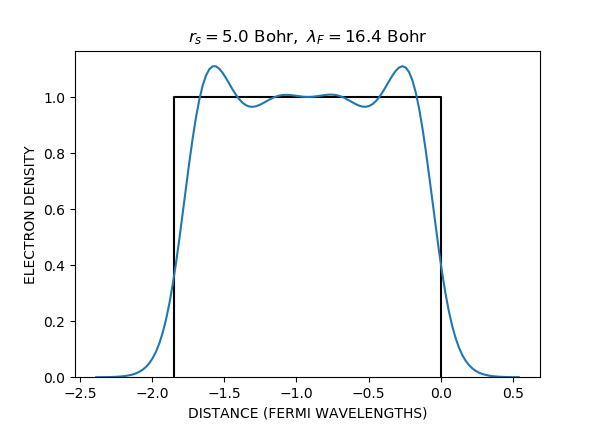
which is reasonably close to the value from Lang and Kohn: 100 ergs/cm\(^2\).
Here is the electron density profile:
# web-page: fig2.png
import numpy as np
import matplotlib.pyplot as plt
from ase.units import Bohr
from gpaw import GPAW
rs = 5.0 * Bohr
calc = GPAW('surface.gpw', txt=None)
density = calc.get_pseudo_density()[0, 0]
h = 0.2
a = 8 * h
v = 3 * a
L = 10 * a
z = np.linspace(0, v + L + v, len(density), endpoint=False)
# Position of surface is between two grid points:
z0 = (v + L - h / 2)
n = 1 / (4 * np.pi / 3 * rs**3)  # electron density
kF = (3 * np.pi**2 * n)**(1.0 / 3)
lambdaF = 2 * np.pi / kF  # Fermi wavelength
plt.figure(figsize=(6, 6 / 2**0.5))
plt.plot([-L / lambdaF, -L / lambdaF, 0, 0], [0, 1, 1, 0], 'k')
plt.plot((z - z0) / lambdaF, density / n)
# plt.xlim(xmin=-1.2, xmax=1)
plt.ylim(ymin=0)
plt.title(r'$r_s=%.1f\ \mathrm{Bohr},\ \lambda_F=%.1f\ \mathrm{Bohr}$' %
          (rs / Bohr, lambdaF / Bohr))
plt.xlabel('DISTANCE (FERMI WAVELENGTHS)')
plt.ylabel('ELECTRON DENSITY')
plt.savefig('fig2.png')
Compare with Fig. 2 in [Lang70]:
Other jellium geometries
For other geometries, one will have to subclass
Jellium, and implement the
get_mask() method:
- class gpaw.jellium.Jellium(charge)[source]
The Jellium object
Initialize the Jellium object
Input: charge, the total Jellium background charge.
The JelliumSlab is one such
example of a subclass of gpaw.jellium.Jellium:
- class gpaw.jellium.JelliumSlab(charge, z1, z2)[source]
The Jellium slab object
Put the positive background charge where z1 < z < z2.
- z1: float
Position of lower surface in Angstrom units.
- z2: float
Position of upper surface in Angstrom units.
N. D. Lang and W. Kohn, Phys. Rev. B 1, 4555-4568 (1970), Theory of Metal Surfaces: Charge Density and Surface Energy, doi: 10.1103/PhysRevB.1.4555