Introduction to PAW
A simple example
We look at the \(2\sigma\)* orbital of a CO molecule: 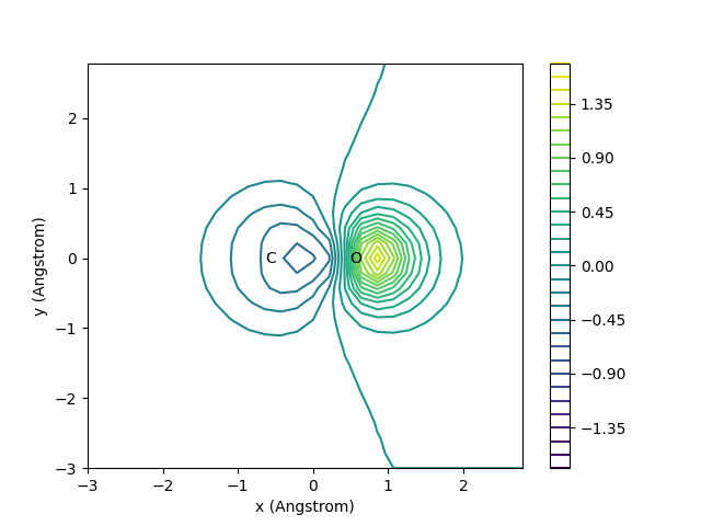
The main quantity in the PAW method is the pseudo wave-function (blue crosses) defined in all of the simulation box:
where \(h\) is the grid spacing and \((i, j, k)\) are the indices of the grid points.
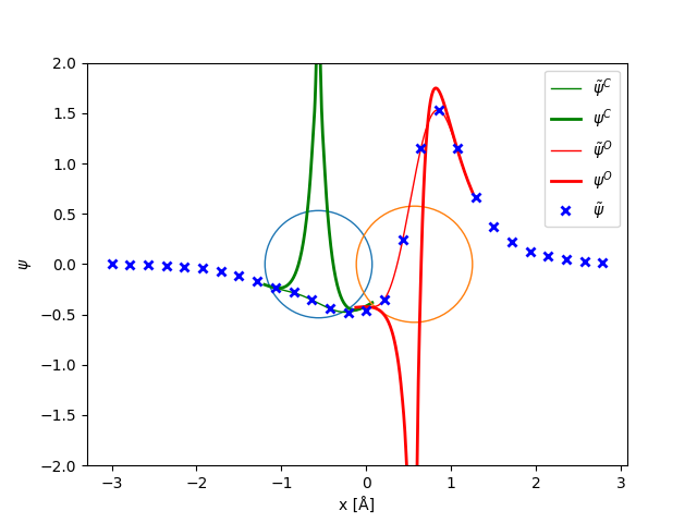
In order to get the all-electron wave function, we add and subtract one-center expansions of the all-electron (thick lines) and pseudo wave-functions (thin lines):
where \(a\) is C or O and \(\phi_i\) and \(\tilde{\phi}_i\) are atom centered basis functions formed as radial functions on logarithmic radial grid multiplied by spherical harmonics.
The expansion coefficients are given as:
Approximations
Frozen core orbitals.
Truncated angular momentum expansion of compensation charges.
Finite number of basis functions and projector functions.
More information on PAW
You can find additional information on the
reports presentations and theses page, or
by reading the paw note.
Script
# creates: 2sigma.png, co_wavefunctions.png
import numpy as np
import matplotlib.pyplot as plt
from ase import Atoms
from ase.units import Bohr

from gpaw import GPAW
from gpaw.spherical_harmonics import Y

L = 6.0
d = 1.13
co = Atoms('CO',
           cell=[L, L, L],
           positions=[(0, 0, 0), (d, 0, 0)])
co.center()
co.calc = GPAW(mode='lcao',
               txt='CO.txt')
e = co.get_potential_energy()
print(co.positions[:, 0] - L / 2)

dpi = 100
C = 'g'
N = 100
for a, pp in enumerate(co.calc.wfs.setups):
    rc = max(pp.rcut_j)
    print(pp.rcut_j)
    x = np.linspace(-rc, rc, 2 * N + 1)
    P_i = co.calc.wfs.kpt_qs[0][0].projections[a][1] / Bohr**1.5
    phi_i = np.empty((len(P_i), len(x)))
    phit_i = np.empty((len(P_i), len(x)))
    i = 0
    for l, phi_g, phit_g in zip(pp.l_j, pp.data.phi_jg, pp.data.phit_jg):
        f = pp.rgd.spline(phi_g, rc + 0.3, l).map(x[N:]) * x[N:]**l
        ft = pp.rgd.spline(phit_g, rc + 0.3, l).map(x[N:]) * x[N:]**l
        for m in range(2 * l + 1):
            ll = l**2 + m
            phi_i[i, N:] = f * Y(ll, 1, 0, 0)
            phi_i[i, N::-1] = f * Y(ll, -1, 0, 0)
            phit_i[i, N:] = ft * Y(ll, 1, 0, 0)
            phit_i[i, N::-1] = ft * Y(ll, -1, 0, 0)
            i += 1
    x0 = co.positions[a, 0] - L / 2
    symbol = co.symbols[a]
    print(symbol, x0, rc)
    plt.plot([x0], [0], 'o', ms=dpi * rc * 2 / 2.33 * 1.3 * Bohr,
             mfc='None', label='_nolegend_')
    plt.plot(x * Bohr + x0, P_i.dot(phit_i), C + '-', lw=1,
             label=r'$\tilde{\psi}^%s$' % symbol)
    plt.plot(x * Bohr + x0, P_i.dot(phi_i), C + '-', lw=2,
             label=r'$\psi^%s$' % symbol)
    C = 'r'

psit = co.calc.get_pseudo_wave_function(band=1)
n = len(psit)
psit2 = psit[:, :, n // 2]
psit1 = psit2[:, n // 2]

x = np.linspace(-L / 2, L / 2, n, endpoint=False)
plt.plot(x, psit1, 'bx', mew=2, label=r'$\tilde{\psi}$')

plt.legend(loc='best')
plt.xlabel('x [Å]')
plt.ylabel(r'$\psi$')
plt.ylim(ymin=-2, ymax=2)
# plt.show()
plt.savefig('co_wavefunctions.png', dpi=dpi)

fig = plt.figure()
ax = fig.add_subplot(111)
m = abs(psit2).max() * 1.1
cax = ax.contour(x, x, psit2.T, np.linspace(-m, m, 31))
ax.text(-d / 2, 0, 'C', ha='center', va='center')
ax.text(d / 2, 0, 'O', ha='center', va='center')
cbar = fig.colorbar(cax)
ax.set_xlabel('x (Angstrom)')
ax.set_ylabel('y (Angstrom)')
# plt.show()
fig.savefig('2sigma.png')