Kohn-Sham wavefunctions of the oxygen atom and CO molecule¶

In this section we will look at the Kohn-Sham wavefunctions of the O atom and CO molecule and compare them to results from molecular orbital theory.

The first script O.py sets up an oxygen atom in a cubic supercell with non-periodic boundary conditions and calculates the total energy. A couple of extra bands (i.e. Kohn-Sham states) are included in the calculation:

from ase import Atoms
from ase.io import write
from gpaw import GPAW

# Oxygen atom:
atom = Atoms('O', cell=[6, 6, 6], pbc=False)
atom.center()

calc = GPAW(mode='fd',
            h=0.2,
            hund=True,  # assigns the atom its correct magnetic moment
            txt='O.txt')

atom.calc = calc
atom.get_potential_energy()

# Write wave functions to gpw file:
calc.write('O.gpw', mode='all')

# Generate cube-files of the orbitals:
for spin in [0, 1]:
    for n in range(calc.get_number_of_bands()):
        wf = calc.get_pseudo_wave_function(band=n, spin=spin)
        write('O.%d.%d.cube' % (spin, n), atom, data=wf)

Towards the end, a .gpw file is written with the Kohn-Sham wavefunctions by calc.write('O.gpw', mode='all') and also some cube files containing individual orbatals are written.
Run the script and check the text-output file. What are the occupation numbers for the free oxygen atom?
The orbitals can be visualized using Mayavi and its mayavi.mlab.contour3d() function and the GPAW-calculators get_pseudo_wave_function() method. Reload the gpw-file and look at one of the orbitals like this:
```
from gpaw import GPAW
from mayavi import mlab
calc = GPAW('O.gpw', txt=None)
lumo = calc.get_pseudo_wave_function(band=2, spin=1)
mlab.contour3d(lumo)
mlab.show()
```
For an alternative way of viewing the orbitals, see Visualizing iso-surfaces.

Can you identify the highest occupied state and the lowest unoccupied state?

How do your wavefunctions compare to atomic s- and p-orbitals?
Make a script where a CO molecule is placed in the center of a cubic unit cell with non-periodic boundary conditions, e.g. of 6 Å. For more accurate calculations, the cell should definitely be bigger, but for reasons of speed, we use this cell here. A grid spacing of around 0.20 Å will suffice. Include a couple of unoccupied bands in the calculation (what is the number of valence electrons in CO?). You can quickly create the Atoms object with the CO molecule by:
```
from ase.build import molecule
CO = molecule('CO')
```
This will create a CO molecule with an approximately correct bond length and the correct magnetic moments on each atom.

Then relax the CO molecule to its minimum energy position. Write the relaxation to a trajectory file and the final results to a .gpw file. The wavefunctions are not written to the .gpw file by default, but can again be saved by writing calc.write('CO.gpw', mode='all'), where calc is the calculator object. Assuming you use opt = QuasiNewton(..., trajectory='CO.traj'), the trajectory can be viewed by:
```
$ ase gui CO.traj
```
Try looking at the file while the optimization is running and mark the two atoms to see the bond length.
As this is a calculation of a molecule, one should get integer occupation numbers - check this in the text output. What electronic temperature was used and what is the significance of this?
Plot the Kohn-Sham wavefunctions of the different wavefunctions of the CO molecule like you did for the oxygen atom.
Can you identify the highest occupied state and the lowest unoccupied state?

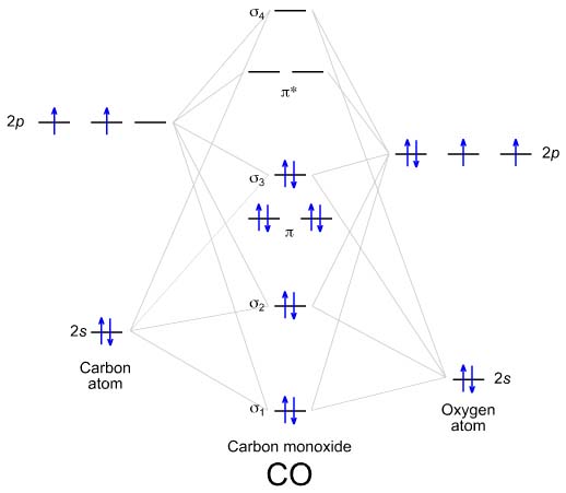
How does your wavefunctions compare to a molecular orbital picture? Try to Identify $\sigma$ and $\pi$ orbitals. Which wavefunctions are bonding and which are antibonding?

Hint

You might find it useful to look at the molecular orbital diagram below, taken from The Chemogenesis Web Book.