Interface to Wannier90
In this tutorial we will briefly scetch the interface to Wannier90. The
tutorial assumes that Wannier90 is installed and wannier90.x,
postw90.x are in your path of executables. We emphasize that this is only
to be regarded as a tutorial on the GPAW interface to Wannier90. Details
and tutorials on the Wannier90 code itself can be found at the Wannier90
home page. For details on the theory the review
paper [1] may be consulted. The interface is
documented in Ref. [2]
Wannier functions of GaAs
As a first example we generate the maximally localized Wannier functions of
GaAs. The ground state is calculated and saved with the following script
GaAs.py. The following
script genrates the maximally localized Wannier functions of the occupied
bands.
import os
from gpaw.wannier90 import Wannier90
from gpaw import GPAW

seed = 'GaAs'

calc = GPAW(seed + '.gpw', txt=None)

w90 = Wannier90(calc,
                seed=seed,
                bands=range(4),
                orbitals_ai=[[], [0, 1, 2, 3]])

w90.write_input(num_iter=1000,
                plot=True)
w90.write_wavefunctions()
os.system('wannier90.x -pp ' + seed)

w90.write_projections()
w90.write_eigenvalues()
w90.write_overlaps()

os.system('wannier90.x ' + seed)
In general Wannier90, needs an .win input file that the user should
write. This contains the \(k\)-point grid, unit cell, positions of atoms, and a
range of parameters specifying the Wannier calculations. Here, we have
provided a helper function write_input_file that provides the most basic
input. In addition, the input file needs to specify the bands contributing to
the wannierization and the initial localized orbitals that the Kohn-Sham
states are projected onto. This is provided with the keywords bands,
which should be a list of bands and orbitals_ai, which should be a list
of lists containing atomic orbital indices for each of the atoms in the
structure. In the example above orbitals_ai an empty list (for the As
atom) and [0, 1, 2, 3] corresponding to the s and p orbitals of the Ga
atom. In this particular example we would like to plot the Wannier functions
and include the plot=True keyword. Altenatively, we could have put
wannier_plot=True in the .win file by hand. For this purpose we also need
the write_wavefunctions function, that writes the periodic part of the
wavefunctions in a special format required by Wannier90.
To proceed, we need lists of nearest neighbor \(k\)-points. This is calculated
with Wannier90 using the wannier90.x -pp GaAs command and stored in
GaAs.nnkp. With these in place, we are ready to perform the largest
calculation of the interface. Namely the initial projector overlaps \(\langle
u_{n\mathbf{k}}|\tilde p^a_i\rangle\) and the overlaps of Bloch states at
neighboring \(k\)-points \(\langle u_{n\mathbf{k}}|u_{n\mathbf{k+b}}\rangle\).
these are stored in GaAs.amn and GaAs.mmn respectively. In addition,
the Kohn-Sham eigenvalues are written to GaAs.eig.
Finally, the Wannier calculation is initiated with wannier90.x GaAs.
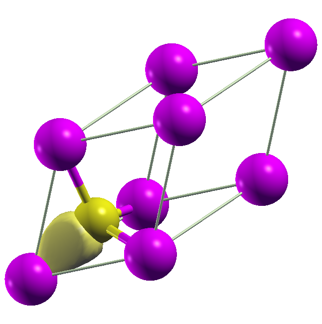
Examining the output GaAs.wout shows that the Wannier functions are Ga
centered s and p orbitals for many iterations. Eventually, additional
localization is obtained by formed four equivalent sp3 orbitals centered at
the bonds. The Wannier90 code actually supports specifying sp3 projectors as
input, but the GPAW interface does not handle this yet. The plot keyword
writes the four Wannier functions in .xsf format, which can be plotted
with xcrysden. An example is shown below.
Fermi surface of Cu
The Wannier functions are extremely useful for calculations requiring a large
number of \(k\)-points. In this respect, we can view the Wannier functions as
comprising a minimal orthonormal tight-binding basis, on which the
Hamiltonian can be diagonalized rapidly on a large number of \(k\)-points. As
an example we consider the Fermi surface of Cu. The ground state Kohn-Sham
structure is rapidly obtained with the script Cu.py on a course
\(k\)-point mesh. In general it is somewhat more difficult to obtain Wannier
functions of metals since the bands below a certain energy has to be
disentangled from higher lying bands. The default energy is 0.1 eV above the
Fermi level. The Wannier functions are generated with the script
import os
from gpaw.wannier90 import Wannier90
from gpaw import GPAW

seed = 'Cu'

calc = GPAW(seed + '.gpw', txt=None)

w90 = Wannier90(calc,
                seed=seed,
                bands=range(20),
                orbitals_ai=[[0, 1, 4, 5, 6, 7, 8]])

w90.write_input(num_iter=1000,
                dis_num_iter=500)

os.system('wannier90.x -pp ' + seed)

w90.write_projections()
w90.write_eigenvalues()
w90.write_overlaps()

os.system('wannier90.x ' + seed)
Note that we now include many more bands (20 lowest bands) than Wannier
functions, which are defined by the number of initial projections. In this
case we use the s orbital, a single p orbital, and the d-band, which has
proven to work well. The dis_num_iter denotes the number of iterations in
the disentangling algorithm. After running the script, add the following
lines to Cu.win:
restart = plot
fermi_surface_plot = True
and do:
wannier90.x Cu
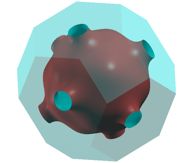
This will diagonalize the Wannier Hamiltonian on a fine \(k\)-mesh and save the
Fermi surface in Cu.bxsf. The result can be plotted with xcrysden and
is shown below. We emphasize that the write_input_file function is just
for generating the basic stuff that should be in the Cu.win input file.
In general this file should be modified according to need before running
wannier90.x.
Berry curvature and anomalous Hall conductivity of Fe
As a final example we calculate the anomalous Hall conductivity of Fe, which
is not easily obtained with GPAW. It can be expressed as a Brillouin zone
integral of the Berry curvature and is an effect of spin-orbit coupling. As
such we need to generate spinorial Wannier functions. The ground state
electronci structure is generated with the script Fe.py.
Note that symmetry has been swtched off in the
calculation, since the interface do not support symmetry reduced \(k\)-points
including spin-orbit coupling at the moment.
This should be trivial to implement though. The
Wannier functions are generated with the script
import os
from gpaw.wannier90 import Wannier90
from gpaw import GPAW

seed = 'Fe'

calc = GPAW('Fe.gpw')

w90 = Wannier90(calc,
                seed=seed,
                bands=range(30),
                spinors=True)

w90.write_input(num_iter=200,
                dis_num_iter=500,
                dis_mix_ratio=1.0,
                dis_froz_max=15.0)

os.system('wannier90.x -pp ' + seed)

w90.write_projections()
w90.write_eigenvalues()
w90.write_overlaps()

os.system('wannier90.x ' + seed)
We have now left out the orbital projections, which means that the default of
all bound projectors are used (s, p and d states in the present case). Note
also that we need to calculate the spin-orbit eigenvalues and wavefunction,
which are supplied as input. After running the script, add the following
lines to Fe.win:
kpath = True
kpath_task = curv+bands
kpath_num_points = 1000
begin kpoint_path
G 0.0 0.0 0.0        H 0.5 -0.5 -0.5
H 0.5 -0.5 -0.5      P 0.75 0.25 -0.25
P 0.75 0.25 -0.25    N 0.5 0.0 -0.5
N 0.5 0.0 -0.5       G 0.0 0.0 0.0
G 0.0 0.0 0.0        H 0.5 0.5 0.5
H 0.5 0.5 0.5        N 0.5 0.0 0.0
N 0.5 0.0 0.0        G 0.0 0.0 0.0
G 0.0 0.0 0.0        P 0.75 0.25 -0.25
P 0.75 0.25 -0.25    N 0.5 0.0 0.0
end kpoint_path
and run:
postw90.x Fe
This will calculate the band structure and Berry curvature along the
specified path. Note that the calculatons is orders of magnitude faster
compared to a standard non self-consistent band structure calculation with
GPAW. It also generates the script Fe-bands+curv_z.py, which can be used
to plot the band structure along with the \(z\)-component of the Berry
curvature. The result is shown below
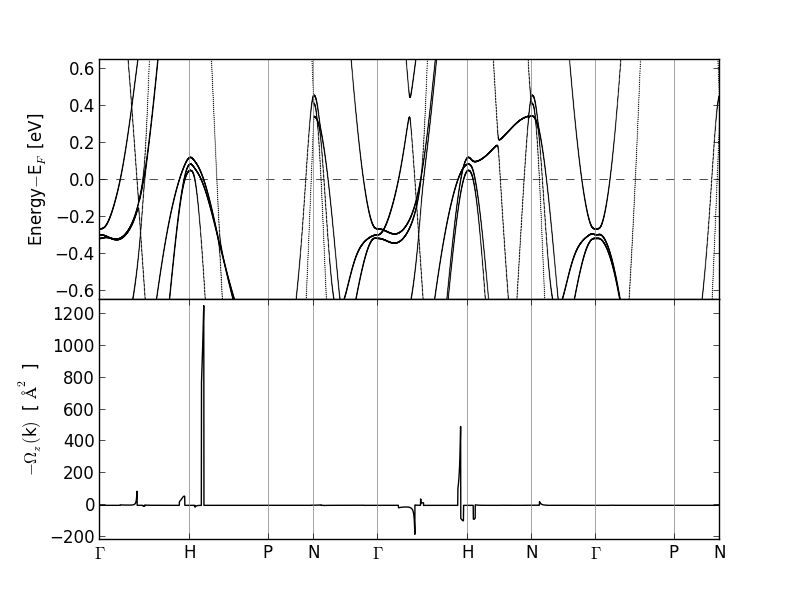
The spiky structure of the Berry curvature makes it highly non-trivial to
converge the anomalous Hall conductivity with respect to \(k\)-points. The
Wannier functions can aid the calculations by performing rapid calculations
on a very fine mesh. To perform the calculation set kpath = False in
Fe.win and add the following lines:
berry = True
berry_task = ahc
berry_kmesh = 50 50 50
Now run postw90.x Fe once more. This calculates the anomalous Hall
conductivity on a \(50\times50\times50\) \(k\)-mesh. The \(z\)-component should be
873 S/cm and can be read from the output file Fe.wpout. This is not too
bad, but one needs to go to much higher \(k\)-point densities to obtain the
converged values of 757 S/cm [3].