Magnon dispersion from the magnetic force theorem
A magnon is a collective spin wave excitation carrying a single unit of spin angular momentum. The magnon quasi-particles can be viewed as the bosons that quantize the fluctuations in the magnetization of a crystal the same way that phonons quantize lattice vibrations. Here we show how to compute the magnon energy dispersion in GPAW, using the magnetic force theorem in a linear response formulation.
Background theory
Classical Heisenberg model
In the classical isotropic Heisenberg model, the magnetization of a crystal is partitioned into distinct magnetic sites with individual magnetic moments \(M_a\) and orientation of the moments \(\mathbf{u}_{ia}\) (unit vector). Here, \(i\) is the unit cell index and \(a\) indexes the magnetic sublattices of the crystal. The system energy is then parametrized in terms of the Heisenberg exchange parameters \(J_{ij}^{ab}\) as follows:
From the exchange parameters, one can compute the magnon dispersion of the system using linear spin wave theory. In particular, the magnon energies \(\hbar\omega_n(\mathbf{q})\), where \(n\) is the mode index, are given as a function of the wave vector \(\mathbf{q}\) by the eigenvalues to the dynamic spin wave matrix:
Here \(\bar{J}^{ab}(\mathbf{q})\) denotes the periodic part of the lattice Fourier transform of the exchange parameters,
where \(\mathbf{R}_i\) refers to the Bravais lattice point corresponding to the \(i\)’th unit cell.
Magnetic force theorem (MFT)
In reference [1], it is shown how the Kohn-Sham Hamiltonian in the local spin-density approximation can be mapped onto a classical isotropic Heisenberg model based on the magnetic force theorem. To do so, it is assumed that the ground state magnetization \(\mathbf{m}(\mathbf{r})=m(\mathbf{r}) \mathbf{u}(\mathbf{r})\) can be treated in the rigid spin approximation,
where \(\Theta(\mathbf{r}\in\Omega_{ia})\) is a unit step function, which is nonzero for positions \(\mathbf{r}\) inside the site volume \(\Omega_{ia}\). In this way, it is the geometry of the sublattice site volumes, that defines what Heisenberg model the DFT problem is mapped onto, and it is not clear a priori that there should exist a unique choice for these geometries.
Once the site geometries have been appropriately chosen, the exchange constants can be calculated in a linear response formulation of the magnetic force theorem,
where all quantities are given in a plane wave basis and matrix/vector multiplication in reciprocal lattice vectors \(\mathbf{G}\) is implied. In this MFT formula for the exchange constants, \(\Omega_{\mathrm{cell}}\) denotes the unit cell volume, \(B^{\mathrm{xc}}(\mathbf{r}) = \delta E_{\mathrm{xc}}^{\mathrm{LSDA}} / \delta m(\mathbf{r})\), \(\chi_{\mathrm{KS}}^{'+-}(\mathbf{q})\) is the reactive part of the static transverse magnetic susceptibility of the Kohn-Sham system, and so-called sublattice site kernels,
have been introduced to encode the sublattice site geometries defined though \(\Omega_{a}=\Omega_{0a}\). For additional details, please refer to [1].
GPAW implementation
In GPAW, the computation of MFT Heisenberg exchange constants is implemented
through the IsotropicExchangeCalculator. The calculator is constructed
from a ChiKSCalculator and a LocalFTCalculator, where the latter
takes care of Fourier transforming \(B^{\mathrm{xc}}(\mathbf{r})\) into
plane-wave components, whereas the former is a separate calculator for
computing the Kohn-Sham transverse magnetic plane wave susceptibility:
Here, \(\Omega\) is the crystal volume, \(\epsilon_{n\mathbf{k}s}\) and \(f_{n\mathbf{k}s}\) the Kohn-Sham eigenvalues and occupation numbers and the plane wave pair densities,
are computed directly from the Kohn-Sham orbitals
\(\psi_{n\mathbf{k}s}(\mathbf{r})\). For more details on the transverse
magnetic susceptibility, PAW corrections to Fourier transforms and their
respective GPAW implementations, please refer to [2]. Specifically,
the ChiKSCalculator evaluates the sum over \(\mathbf{k}\)-points by point
integration on the Monkhorst-Pack grid specified by an input ground state
DFT calculation. Because of this, it only accepts wave vectors \(\mathbf{q}\)
that are commensurate with the underlying \(\mathbf{k}\)-point grid.
Furthermore, it takes input arguments ecut and nbands in the
constructor, specifying the plane wave energy cutoff and number of bands in
the band summation respectively.
The IsotropicExchangeCalculator uses the ChiKSCalculator instance
from which it is initialized to compute the reactive part of the
susceptibility,
in the static limit \(\omega=0\) and without broadening \(\eta=0\) for a given
wave vector \(\mathbf{q}\). With this in hand, it uses a supplied
SiteKernels instance defining the sublattice site geometries to compute
the exchange constants \(\bar{J}^{ab}(\mathbf{q})\). At present, spherical,
cylindrical and parallelepipedic site kernel geometries are supported
through the SphericalSiteKernels, CylindricalSiteKernels and
ParallelepipedicSiteKernels classes.
When using the GPAW code for computing MFT Heisenberg exchange constants, please reference both of the works [1] and [2].
Example 1 (Introductory): bcc-Fe
In this first example, we will compute the magnon dispersion of iron, which is an itinerant ferromagnet with a single magnetic atom in the unit cell.
First, you should download the ground state calculation script
Fe_gs.py
and run it using a cluster available to you. Resource estimate: 10
minutes on a 40 core node. The script will perform a LSDA ground state
calculation and store all its data to a file, Fe_all.gpw.
Secondly, download and run the
Fe_mft.py
script to perform the MFT calculation of the Heisenberg exchange
parameters. Resource estimate: 30 minutes on a 40 core node. The script
computes the exchange constants on the high-symmetry path G-N-P-G-H
using two different site geometries:
Spherical site volumes centered on the Fe atoms with varying radii.
Parallelepipedic site volumes filling out the entire unit cell.
After the calculation, the \(\mathbf{q}\)-point path, spherical radii
and exchange constants are stored in separate .npz files.
Now it is time to visualize the data. GPAW distributes functionality to
compute the magnon dispersion for a single site ferromagnet from its
isotropic exchange constants \(\bar{J}(\mathbf{q})\), namely through the
method calculate_single_site_magnon_energies. In the script
Fe_plot_magnons_vs_rc.py,
the magnon energy of iron in the high-symmetry points N, P and H is
plotted as a function of the spherical site radii, resulting in the
following figure:
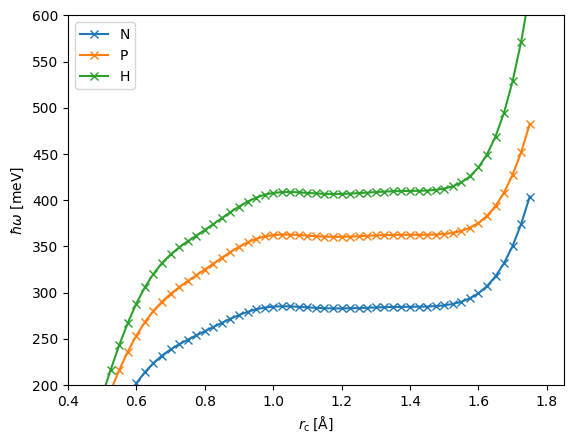
Although there does not exist a unique definition of the correct magnetic site volumes, there clearly seems to be a range of spherical cutoff radii \(r_{\mathrm{c}}\in[1.0\,\mathrm{Å}, 1.5\,\mathrm{Å}]\) in which the MFT magnon energy for a given wave vector \(\mathbf{q}\) is well defined! It is not clear a priori that there always exists such a range, why it should always be double-checked, when performing MFT calculations.
Finally, we use the script
Fe_plot_magnon_dispersion.py,
to plot the magnon dispersion along the entire band path for both of our
chosen site geometries:
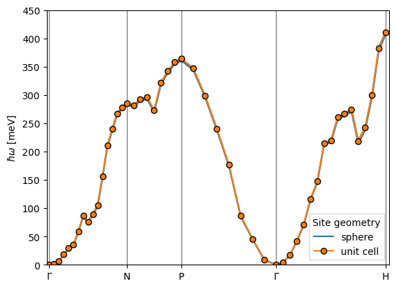
Even though we are showing the entire range of magnon energies for \(r_{\mathrm{c}}\in[1.0\,\mathrm{Å}, 1.5\,\mathrm{Å}]\), the spread is not visible on the frequency scale of the actual magnon dispersion, why we can conclude that the MFT magnon dispersion is well defined for the entire Brillouin Zone! This is confirmed by the calculations using the parallelepipedic site volumes, which yields identical results.
Example 2 (Advanced): hcp-Co
In the second example we will consider hcp-Co, which is also an itinerant ferromagnet, but this time with two magnetic atoms in the unit cell. This means that we will have two magnetic sublattices and two magnon modes, the usual acoustic Goldtone mode and an optical mode.
Again, we start off by calculating the LSDA ground state using the script
Co_gs.py
(resource estimate: 15 minutes on a 40 core node). However, this time we do
not save the Kohn-Sham orbitals as they can take up a significant amount of
disc space (hundreds of GB) for large systems. Instead, we will recalculate
the orbitals as the first thing in the MFT calculation script
Co_mft.py.
Typically, this will not take much extra time. In fact, it is (depending on
your hard disk/file system) sometimes faster, as file io can be a real
bottle-neck when working with hundreds of GBs of data.
Following the recalculation of the Kohn-Sham orbitals,
Co_mft.py
computes the Co MFT Heisenberg exchange constants for the band path
G-M-K-G-A using several different spatial partitionings into magnetic sites:
A partitioning where the two cobalt atoms are assigned each a spherical site, but where only one of the spherical cutoff radii is varried.
A similar partitioning with spheres of varying, but equal radii.
A partitioning with only one sublattice that fills out the entire unit cell.
A partitioning with a single sublattice of cylindrical shape encapsulating both cobalt atoms in the unit cell.
Resource estimate: 2.5 hours on a 40 cores node.
We kick off our analysis of the results by computing the magnon mode
energies using the build-in function calculate_fm_magnon_energies and
plotting them at the high-symmetry points as a function of cutoff radius in
the model of equally sized spherical sites. Excecuting the plotting script
Co_plot_magnons_vs_rc.py,
results in the following figure:
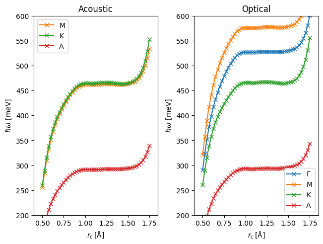
Once again there seems to be a well defined range of spherical radii,
\(r_{\mathrm{c}}\in[1.0\,\mathrm{Å}, 1.4\,\mathrm{Å}]\), within which the
magnon mode energies are constant (well defined). Using the script
Co_plot_magnon_dispersion.py,
we may then plot the full magnon dispersion for spheres inside this range,
along with the magnon dispersion resulting from the other (more
experimental) site kernel definitions:
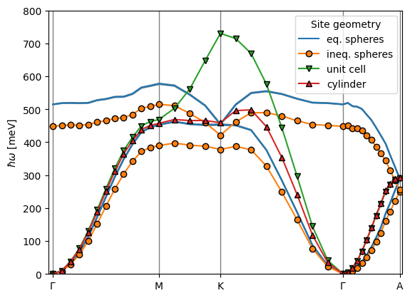
In the model with two spherical sites of inequal radii (0.6 Å and 1.2 Å respectively), the magnon bandwidth is decreased compared to the appropriate model of equivalent spherical sites because some of the magnetization on one of the cobalt atoms has been neglected in the model. However, this is not all. We have also broken the magnon mode degeneracy at the K-point because the magnetic sublattices in the Heisenberg model are no longer equivalent!
For the two Heisenberg models with only a single magnetic sublattice, we can only get an estimate of the acoustic magnon mode dispersion. However, in the long wavelength limit \(\mathbf{q}\rightarrow 0\) the magnetic moment on the two cobalt atoms inside the unit cell will precess in-phase for an acoustic spin-wave, why both of the single sublattice models provide reasonable results in this limit. Interestingly, both models actually also provide a good describtion of the acoustic magnon dispersion on the entire G-M path, a conclusion extending even all the way to the K-point in the case of a cylindrical site volume.
Excercises
Now it is your own turn to experiment with GPAW’s MFT module. To get you started, here are some suggestions:
Compute and plot the iron magnon dispersion as a function of
The parallelepipedic site volume
The cylindrical site orientation, height and radius
Compute and plot the cobalt magnon dispersion
Using a cylindrical site geometry for one cobalt atom and a spherical geometry for the other
Using two equivalent parallelepipeds for the two cobalt sites
Compute and plot the magnon dispersion of your favorite ferromagnet