Spin spiral calculations
In this tutorial we employ the Generalized Bloch’s Theorem (gBT) approach to calculate the spin spiral ground-state [1]. In this approach we can choose any wave vector of the spin spiral \(\mathbf{q}\), and rotate the spin degrees through the periodic boundary conditions accordingly. This rotation can be included in Bloch’s theorem by applying a combined translation and spin rotation to the wave function at the boundaries. Then we get the generalized Bloch’s theorem,
where \(u^{\uparrow}_{\mathbf{q},\mathbf{k}}(\mathbf{r})\) and \(u^{\downarrow}_{\mathbf{q},\mathbf{k}}(\mathbf{r})\) are spin dependent and periodic Bloch functions modulated by the spin rotation matrix
which act as an enveloping function together with the standard Bloch envelope \(e^{i\mathbf{k}\cdot\mathbf{r}}\). This wavefunction ansatz make the magnetic field rotate around the z-axis while leaving the density unchanged as
where \(\mathbf{a}\) are lattice translations. The magnetization direction follows the direction of the magnetic field when the LDA exchange-functional is used. These are called flat spin spirals. There is nothing special about the \(xy\)-plane, used here, since spin-orbit is neglected at this stage, the spin spiral is invariant under any global spinor rotation. The reward is that we can simulate any incommensurate spin spiral of this type in the chemical unit cell.
The initial magnetization is a input parameter, and when the gBT is applied the magnetic moments should correspond to the non-periodic real space structure. As an example consider making a spin spiral calculation in a 1D chain. The spin structure with order parameter \(q = [0.25, 0, 0]\) requires a 4 times enlarged supercell. The input magnetic moments at each site will be rotated by 90 degrees such that \(\mathbf{m}_1=[m, 0, 0], \mathbf{m}_2=[0, m, 0], \mathbf{m}_3=[-m, 0, 0], \mathbf{m}_1=[0, -m, 0]\). The corresponding spin spiral calculation could be done in a calculation with only one magnetic atom, however for illustrative purposes, suppose that we have a unit cell with two atoms then the magnetic moments initialized to \(\mathbf{m}_1=[m, 0, 0], \mathbf{m}_2=[0, m, 0]\). (Note that the alternative would have been to initalize them in parallel, and then rely on \(U_\mathbf{q}(\mathbf{r})\) to do the rotation, however this is not applied to the input moments because \(U_\mathbf{q}(\mathbf{r})\) is absorbed into the projector overlap functions). This magnetization is expected to be found during the self-consistent cycle, however choosing it as the initial magnetic moments can significantly improve convergence.
The z-component being zero is not strictly enforced. Thus, convergence to conical spin spirals is in principle possible if initialized with components both in the \(xy\) plane and in the \(z\) direction. However, typically the magnetization will converge to a collinear state in along the z-axis or the flat spiral in the \(xy\)-plane, depending on the initial angle provided.
There are some limitations associated with these wave functions, because we assume spin structure to decouple from the lattice such that the density matrix is invariant under the spin rotation. In order for this to be the case, we can only apply spin orbit coupling perturbatively [2], and not as part of the self consistent calculation. Furthermore, with the density being invariant under the this spinor rotation, so will also the z-component of the magnetization. This can be understood by looking at the magnetization density \(\tilde{\rho} = I_2\rho + \sigma\cdot m\) under the spin spiral rotation, where one sees that the entire diagonal is left invariant. Thus we are limited to spiral structures which have magnetization vectors
Ground state of Monolayer \(\text{NiI}_2\)
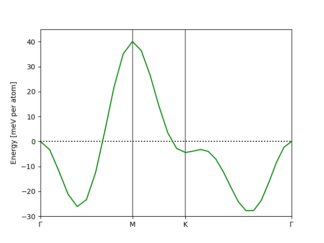
The nickel halide \(\text{NiI}_2\) is a van der waals bonded crystal, where each layers is a 1T monolayer. Thus the nickel form a triangular lattice, which is an interesting platform because magnetic frustration. Particularly one finds that multiple competing interactions in the heisenberg picture can the cause for stabilizing an incommensurate spin spiral ground state \(q \approx 1/7\) that is found in experiments. We can predict using DFT calculations, however if one were to use a supercell approach one would have to compare energies of many large supercells approximating the wavelength. Here we scan the spin spiral groundstate in a systematic way along the high-symmetry bandpath of the crystal. This is done using the following script.
from ase.build import mx2
from gpaw.new.ase_interface import GPAW
import numpy as np

atoms = mx2('NiI2', kind='1T', a=3.969662131560825,
            thickness=3.027146598949815, vacuum=4)

# Align the magnetic moment in the xy-plane
magmoms = [[1, 0, 0], [0, 0, 0], [0, 0, 0]]
ecut = 600
k = 6

# Construct list of q-vectors
path = atoms.cell.bandpath('GMKG', npoints=31).kpts

energies_q = []
magmoms_q = []

for i, q_c in enumerate(path):
    # Spin-spiral calculations require non-collinear calculations
    # without symmetry or spin-orbit coupling
    calc = GPAW(mode={'name': 'pw',
                      'ecut': ecut,
                      'qspiral': q_c},
                xc='LDA',
                mixer={'backend': 'pulay',
                       'beta': 0.05,
                       'method': 'sum',
                       'nmaxold': 5,
                       'weight': 100},
                symmetry='off',
                parallel={'domain': 1, 'band': 1},
                magmoms=magmoms,
                kpts={'density': 6.0, 'gamma': True},
                txt=f'gsq-{i:02}.txt')
    atoms.calc = calc
    energy = atoms.get_potential_energy()
    calc.write(f'gsq-{i:02}.gpw')
    magmom = atoms.calc.dft.magmoms()[0]
    energies_q.append(energy)
    magmoms_q.append(np.linalg.norm(magmom))

energies_q = np.array(energies_q)
magmoms_q = np.array(magmoms_q)
np.savez('data.npz', energies=energies_q, magmoms=magmoms_q)
As a results we find that two minima can be found along both orthogonal directions, indeed one can find paths in the \(\mathbf{q}\)-space and find the minima are seperated by a very small barrier of about 2meV.
The spin spiral groundstate breaks a lot of the symmetries in the crystal spacegroup, for example \(\text{NiI}_2\) is a centrosymmetric crystal but the inversion symmetry is broken by the spin spiral order. The electronic density can then polarize as a consequence of the magnetic order, which is denoted a type II multiferroric material. Although some mirror symmetries might persist, depending on the orientation of the spin spiral plane. The plane orientation is usually the normal plane vector \(\mathbf{n} = (\theta, \varphi)\). The normal plane vector can be determined self-consistently in a supercell calculation, however converging exact angles can be very tricky. Instead we can leverege the small spin spiral groundstate, do a scan of scan of \(\mathbf{n}\) non-self-consistently using the projected spin-orbit approximation [2]. In the following script we do such a scan, but limited to the upper half hemisphere of points, since the lower is related by time-reversal symmetry.
import numpy as np
from gpaw.occupations import create_occ_calc
from gpaw.spinorbit import soc_eigenstates
from gpaw.new.ase_interface import GPAW


def sphere_points(distance=None):
    '''Calculates equidistant points on the upper half sphere

    Returns list of spherical coordinates (thetas, phis) in degrees

    Modified from:
        M. Deserno 2004 If Polymerforshung (Ed.) 2 99
    '''

    import math
    N = math.ceil(129600 / (math.pi) * 1 / distance**2)
    if N <= 1:
        return np.array([0.]), np.array([0.])

    A = 4 * math.pi
    a = A / N
    d = math.sqrt(a)

    # Even number of theta angles ensure 90 deg is included
    Mtheta = round(math.pi / (2 * d)) * 2
    dtheta = math.pi / Mtheta
    dphi = a / dtheta
    points = []

    # Limit theta loop to upper half-sphere
    for m in range(Mtheta // 2 + 1):
        # m = 0 ensure 0 deg is included, Mphi = 1 is used in this case
        theta = math.pi * m / Mtheta
        Mphi = max(round(2 * math.pi * math.sin(theta) / dphi), 1)
        for n in range(Mphi):
            phi = 2 * math.pi * n / Mphi
            points.append([theta, phi])
    thetas, phis = np.array(points).T

    if not any(thetas - np.pi / 2 < 1e-14):
        import warnings
        warnings.warn('xy-plane not included in sampling')

    return thetas * 180 / math.pi, phis * 180 / math.pi


energies = np.load('data.npz')['energies']
minimum = np.argmin(energies)

theta_tp, phi_tp = sphere_points(distance=1)
calc = GPAW(f'gsq-{minimum:02}.gpw')
occcalc = create_occ_calc({'name': 'fermi-dirac', 'width': 0.001})
soc_tp = np.array([])
for theta, phi in zip(theta_tp, phi_tp):
    en_soc = soc_eigenstates(calc=calc, projected=True, theta=theta, phi=phi,
                             occcalc=occcalc).calculate_band_energy()
    soc_tp = np.append(soc_tp, en_soc)

np.savez('soc_data.npz', soc=soc_tp, theta=theta_tp, phi=phi_tp)
In order to plot the scan of the spherical surface, we choose here to do a stereographic projection of the half-sphere, which puts the out-of-plane direction \(z\) in the center of a circle. The radial coordinate of the circle corresponds to the \(\theta\) direction and the angular coordinate to the \(\phi\) direction. We find that the spin-orbit energy landscape has a hard axis and a very flat easy plane as seen below. Besides the contour displayed on the colorbar, we also show the points within \(50\mu eV\) and \(1\mu eV\) of the minimum in midnight blue and black respectively. The z-axis is shown as a black dot in the middle of the stereographic plot, and the white dot is the minimum which corresponds to \(\mathbf{n} = (33, 301)\) degrees with an uncertainty of 1 degree.
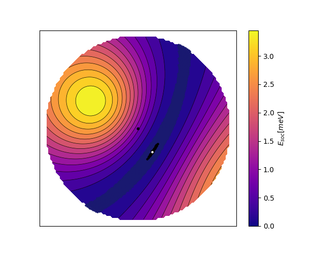
(see plot_soc.py)