Calculating RPA correlation energies
The Random Phase Approximation (RPA) can be used to derive a non-local expression for the ground state correlation energy. The calculation requires a large number of unoccupied bands and is significantly heavier than standard DFT calculation using semi-local exchange-correlation functionals. However, when combined with exact exchange the method has been shown to give a good description of van der Waals interactions and a decent description of covalent bonds (slightly worse than PBE).
For more details on the theory and implementation we refer to RPA correlation energy. Below we give examples on how to calculate the RPA atomization energy of \(N_2\) and the correlation energy of graphene an a Cu(111) surface. Note that some of the calculations in this tutorial will need a lot of CPU time and is essentially not possible without a supercomputer.
Example 1: Atomization energy of N2
The atomization energy of \(N_2\) is overestimated by typical GGA functionals, and the RPA functional seems to do a bit better. This is not a general trend for small molecules, however, typically the HF-RPA approach yields too small atomization energies when evaluated at the GGA equilibrium geometry. See for example Furche [1] for a table of atomization energies for small molecules calculated with the RPA functional.
Ground state calculation
First we set up a ground state calculation with lots of unoccupied bands. This is done with the script:
from ase.optimize import BFGS
from ase.build import molecule
from ase.parallel import paropen
from gpaw import GPAW, PW
from gpaw.hybrids.energy import non_self_consistent_energy as nsc_energy

# N
N = molecule('N')
N.cell = (6, 6, 7)
N.center()
calc = GPAW(mode=PW(600, force_complex_dtype=True),
            symmetry='off',
            nbands=16,
            maxiter=300,
            xc='PBE',
            hund=True,
            txt='N_pbe.txt',
            parallel={'domain': 1},
            convergence={'density': 1.e-6})

N.calc = calc
E1_pbe = N.get_potential_energy()

calc.write('N.gpw', mode='all')

E1_hf = nsc_energy('N.gpw', 'EXX').sum()

# calc.diagonalize_full_hamiltonian(nbands=4800)
calc.diagonalize_full_hamiltonian(nbands=None)
calc.write('N.gpw', mode='all')

# N2
N2 = molecule('N2')
N2.cell = (6, 6, 7)
N2.center()
calc = GPAW(mode=PW(600, force_complex_dtype=True),
            symmetry='off',
            nbands=16,
            maxiter=300,
            xc='PBE',
            txt='N2_pbe.txt',
            parallel={'domain': 1},
            convergence={'density': 1.e-6})

N2.calc = calc
dyn = BFGS(N2)
dyn.run(fmax=0.05)
E2_pbe = N2.get_potential_energy()

calc.write('N2.gpw', mode='all')

E2_hf = nsc_energy('N2.gpw', 'EXX').sum()

with paropen('PBE_HF.dat', 'w') as fd:
    print('PBE: ', E2_pbe - 2 * E1_pbe, file=fd)
    print('HF: ', E2_hf - 2 * E1_hf, file=fd)

# calc.diagonalize_full_hamiltonian(nbands=4800)
calc.diagonalize_full_hamiltonian(nbands=None)
calc.write('N2.gpw', mode='all')
which takes on the order of 3-4 CPU hours. The script generates N.gpw and
N2.gpw which are the input to the RPA calculation. The PBE and
non self-consistent Hartree-Fock energy is also calculated and written to the
file PBE_HF.dat. Be aware that using symmetries (i. e. not using symmetry='off'
in the calculator) may cause problems if you want to calculate non self-consistent
HF energies for atoms and molecules.
Converging the frequency integration
We will start by making a single RPA calculation with extremely fine frequency sampling. The following script returns the integrand at 2000 frequency points from 0 to 1000 eV from a cutoff of 50 eV.
from ase.parallel import paropen
from gpaw.xc.rpa import RPACorrelation
import numpy as np

dw = 0.5
frequencies = np.array([dw * i for i in range(200)])
weights = len(frequencies) * [dw]
weights[0] /= 2
weights[-1] /= 2
weights = np.array(weights)

rpa = RPACorrelation('N2.gpw',
                     txt='frequency_equidistant.txt',
                     frequencies=frequencies,
                     weights=weights,
                     ecut=[50])
Es = rpa.calculate()
Es_w = rpa.E_w

with paropen('frequency_equidistant.dat', 'w') as fd:
    for w, E in zip(frequencies, Es_w):
        print(w, E.real, file=fd)
The correlation energy is obtained as the integral of this function divided by \(2\pi\) and yields -6.62 eV. The frequency sampling is dense enough so that this value can be regarded as “exact” (but not converged with respect to cutoff energy, of course). We can now test the Gauss-Legendre integration method with different number of points using the same script but now specifying the Gauss-Legendre parameters instead of a frequency list:
rpa = RPACorrelation(calc,
                     nfrequencies=16,
                     frequency_max=800.0,
                     frequency_scale=2.0)
This is the default parameters for Gauss-legendre integration. The nfrequencies keyword specifies the number of points, the frequency_max keyword sets the value of the highest frequency (but the integration is always an approximation for the infinite integral) and the frequency_scale keyword determines how dense the frequencies are sampled close to \(\omega=0\). The integrals for different number of Gauss-Legendre points is shown below as well as the integrand evaluated at the fine equidistant frequency grid.
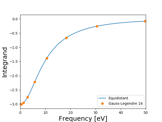

It is seen that using the default value of 16 frequency points gives a result which is very well converged (to 0.1 meV). Below we will simply use the default values although we could perhaps use 8 points instead of 16, which would half the total CPU time for the calculations. In this particular case the result is not very sensitive to the frequency scale, but if the there is a non-vanishing density of states near the Fermi level, there may be much more structure in the integrand near \(\omega=0\) and it is important to sample this region well. It should of course be remembered that these values are not converged with respect to the number of unoccupied bands and plane waves.
Extrapolating to infinite number of bands
To calculate the atomization energy we need to obtain the correlation energy as a function of cutoff energy and extrapolate to infinity as explained in RPA correlation energy [2]. This is accomplished with the script:
from ase.parallel import paropen
from ase.units import Hartree
from gpaw.xc.rpa import RPACorrelation

rpa = RPACorrelation('N.gpw', nblocks=8,
                     txt='rpa_N.txt', ecut=400)
E1_i = rpa.calculate()

rpa = RPACorrelation('N2.gpw', nblocks=8,
                     txt='rpa_N2.txt', ecut=400)
E2_i = rpa.calculate()
ecut_i = rpa.ecut_i

f = paropen('rpa_N2.dat', 'w')
for ecut, E1, E2 in zip(ecut_i, E1_i, E2_i):
    print(ecut * Hartree, E2 - 2 * E1, file=f)
f.close()
which calculates the correlation part of the atomization energy with the
bands and plane waved corresponding to the list of cutoff energies. Note that
the default value of frequencies (16 Gauss-Legendre points) is used. The
script takes on the order of two CPU hours, but can be efficiently
parallelized over kpoints, spin and bands. If memory becomes and issue, it
may be an advantage to specify parallelize over G-vectors, which is
done by specifying nblocks=N. The result is written to
rpa_N2.dat and can be visualized with the script:
# web-page: extrapolate.png, N2-data.csv
import numpy as np
import matplotlib.pyplot as plt
from gpaw.utilities.extrapolate import extrapolate
from pathlib import Path

a = np.loadtxt('rpa_N2.dat')
ext, A, B, sigma = extrapolate(a[:, 0], a[:, 1], reg=3, plot=False)
plt.plot(a[:, 0]**(-1.5), a[:, 1], 'o', label='Calculated points')
es = np.array([e for e in a[:, 0]] + [10000])
plt.plot(es**(-1.5), A + B * es**(-1.5), '--', label='Linear regression')

t = [int(a[i, 0]) for i in range(len(a))]
plt.xticks(a[:, 0]**(-1.5), t, fontsize=12)
plt.axis([0., 150**(-1.5), None, -4.])
plt.xlabel('Cutoff energy [eV]', fontsize=18)
plt.ylabel('RPA correlation energy [eV]', fontsize=18)
plt.legend(loc='lower right')
plt.savefig('extrapolate.png')

pbe, hf = (-float(line.split()[1])
           for line in Path('PBE_HF.dat').read_text().splitlines())
rpa = -A
Path('N2-data.csv').write_text(
    'PBE, HF, RPA, HF+RPA, Experimental\n'
    f'{pbe:.2f}, {hf:.2f}, {rpa:.2f}, {hf + rpa:.2f}, 9.89\n')
The figure is shown below
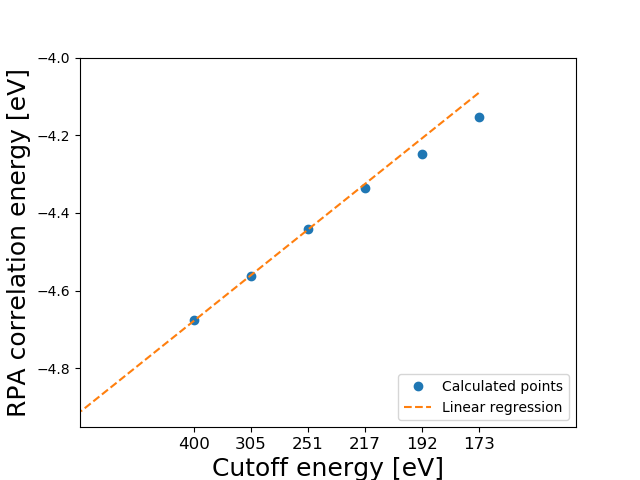
Note that the extrapolate function can also be used to visualize the result by setting plot=True. The power law scaling is seen to be very good at the last three points and the extrapolated results is obtained using linear regression on the last three points (reg=3). We find an extrapolated value of -4.91 eV for the correlation part of the atomization energy. The results are summarized below (all values in eV)
PBE |
HF |
RPA |
HF+RPA |
Experimental |
10.60 |
4.84 |
4.91 |
9.75 |
9.89 |
It should be noted that in general, the accuracy of RPA is comparable to (or worse) that of PBE calculations and N2 is just a special case where RPA performs better than PBE. The major advantage of RPA is the non-locality, which results in a good description of van der Waals forces. The true power of RPA thus only comes into play for systems where dispersive interactions dominate.
Example 2: Adsorption of graphene on metal surfaces
As an example where dispersive interactions are known to play a prominent role, we consider the case of graphene adsorbed on a Cu(111) surface [3] and [4].
from pathlib import Path

from ase import Atoms
from ase.build import fcc111
from gpaw import GPAW, PW, FermiDirac, MixerSum, Davidson
from gpaw.hybrids.energy import non_self_consistent_energy as nsc_energy
from gpaw.mpi import world
from gpaw.xc.rpa import RPACorrelation

# Lattice parametes of Cu:
d = 2.56
a = 2**0.5 * d
slab = fcc111('Cu', a=a, size=(1, 1, 4), vacuum=10.0)
slab.pbc = True

# Add graphite (we adjust height later):
slab += Atoms('C2',
              scaled_positions=[[0, 0, 0],
                                [1 / 3, 1 / 3, 0]],
              cell=slab.cell)


def calculate(xc: str, d: float) -> float:
    slab.positions[4:6, 2] = slab.positions[3, 2] + d
    tag = f'{d:.3f}'
    if xc == 'RPA':
        xc0 = 'PBE'
    else:
        xc0 = xc
    slab.calc = GPAW(xc=xc0,
                     mode=PW(800),
                     basis='dzp',
                     eigensolver=Davidson(niter=4),
                     nbands='200%',
                     kpts={'size': (12, 12, 1), 'gamma': True},
                     occupations=FermiDirac(width=0.05),
                     convergence={'density': 1e-5},
                     parallel={'domain': 1},
                     mixer=MixerSum(0.05, 5, 50),
                     txt=f'{xc0}-{tag}.txt')
    e = slab.get_potential_energy()

    if xc == 'RPA':
        e_hf = nsc_energy(slab.calc, 'EXX').sum()

        slab.calc.diagonalize_full_hamiltonian()
        slab.calc.write(f'{xc0}-{tag}.gpw', mode='all')

        rpa = RPACorrelation(f'{xc0}-{tag}.gpw',
                             ecut=[200],
                             txt=f'RPAc-{tag}.txt',
                             skip_gamma=True,
                             frequency_scale=2.5)
        e_rpac = rpa.calculate()[0]
        e = e_hf + e_rpac

        if world.rank == 0:
            Path(f'{xc0}-{tag}.gpw').unlink()
            with open(f'RPA-{tag}.result', 'w') as fd:
                print(d, e, e_hf, e_rpac, file=fd)

    return e


if __name__ == '__main__':
    import sys
    xc = sys.argv[1]
    for arg in sys.argv[2:]:
        d = float(arg)
        calculate(xc, d)
Note that besides diagonalizing the full Hamiltonian for each distance, the script calculates the EXX energy at the self-consistent PBE orbitals and writes the result to a file. It should also be noted that the k-point grid is centered at the Gamma point, which makes the q-point reduction in the RPA calculation much more efficient. In general, RPA and EXX is more sensitive to Fermi smearing than semi-local functionals and we have set the smearing to 0.01 eV. Due to the long range nature of the van der Waals interactions, a lot of vacuum have been included above the slab. The calculation should be parallelized over spin and irreducible k-points.
The RPA calculations are rather time consuming (~50 CPU hours per distance point), but can be parallelized very efficiently over bands, k-points (default) and frequencies (needs to be specified). Here we have changed the frequency scale from the default value of 2.0 to 2.5 to increase the density of frequency points near the origin. We also specify that the Gamma point (in q) should not be included since the optical limit becomes unstable for systems with high degeneracy near the Fermi level. The restart file contains the contributions from different q-points, which is read if a calculation needs to be restarted.
In principle, the calculations should be performed for a range of cutoff energies and extrapolated to infinity as in the example above. However, energy differences between systems with similar electronic structure converges much faster than absolute correlation energies and a reasonably converged potential energy surface can be obtained using a fixed cutoff of 200 eV for this system.
The result is shown in the figure below along with LDA, PBE and vdW-DF results.
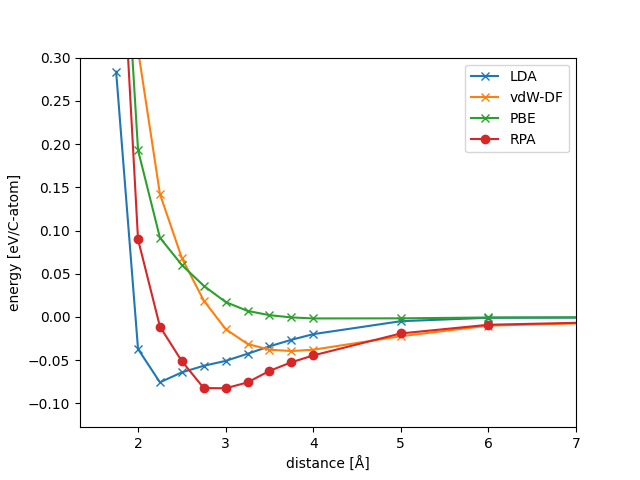
LDA predicts adsorption at 2 Å from the metal slab, but do not include van der Waals attraction. The van der Waals functional shows a significant amount of dispersive interactions far from the slab and predicts a physisorbed minimum 3.75 Å from the slab. RPA captures both covalent and dispersive interactions and the resulting potential energy surface is a delicate balance between the two types of interactions.