Calculating the formation energies of charged defects

Introduction

The energy required to form a point defect in an otherwise pristine sample is usually calculated using the so-called Zhang-Northrup formula [1]:

\[E^f[X^q] = E[X^q] - E_0 - \sum_i\mu_in_i + q (\epsilon_v + \epsilon_F)\]

In this formula, \(X\) labels the type of defect (e.g. a gallium vacancy \(\mathrm{V_{Ga}}\) or zinc interstitial \(\mathrm{Zn_i}\)) and \(q\) its charge state, i.e. the net charge contained in some volume surrounding the defect. \(q\) is defined such that \(q=-1\) for an electron. \(E[X^q]\) is the total energy of the sample with the defect, and \(E_0\) the energy of the pristine (bulklike) sample. In general, we form the defect by changing the number of (neutral) atoms of species \(i\) in the sample by \(n_i\); the change in energy due to this addition (or removal) of atoms is quantified by the chemical potentials \(\mu_i\) of each species. Similarly, if we require the addition or removal of electrons to form the defect (i.e. to obtain a nonzero charge state) we also change the energy according to the chemical potential of the electrons as \(N_e \mu_e\). \(N_e\) is simply related to \(q\) as \(N_e = -q\), while conventionally \(\mu_e\) is written in terms of a “Fermi Energy” referenced to the valence band maximum \(\epsilon_v\), i.e. \(\mu_e = \epsilon_v + \epsilon_F\). Taking everything together, the formation energy can thus be interpreted as the difference in total energy of the sample containing a defect and the total energy of all the constituents required to form the defect (the pristine sample, atoms and electrons). In general one expects a defect formation energy to be positive, so that it costs energy to make a defect. The formation energy will also depend on the chemical potentials of the atoms and of the electrons, reflecting the growth conditions of the sample.

Within periodic boundary conditions, the quantity \(E[X^q] - E_0\) is obtained by constructing supercells of the pristine unit cell, and then calculating the difference in total energies of the supercells with and without the defect. In the limit of an infinitely large supercell, the dilute limit of a single, isolated defect should be achieved. In practice however, a variety of finite size effects can lead to slow convergence with supercell size [2]. In the case of nonzero charge states, the electrostatic interaction between the periodically repeated array of defects leads to particularly slow convergence. In this tutorial, we apply the method proposed by Freysoldt, Neugebauer and Van de Walle (FNV) [3] to correct for this effect in a bulk system, namely the triply charged gallium vacancy in GaAs, as well as in a 2D system.

Theoretical background: The FNV scheme

Here we outline the FNV approach to correcting for the electrostatic interactions; more details can be found in [3]. A practical example is given in the next section. The electrostatic energy of a periodically repeated charged system is divergent. Therefore, the calculation of \(E[X^q]\) in periodic boundary conditions is only possible if one adds a homogeneous neutralising background charge of density \(-q/\Omega\) (where \(\Omega\) is the volume of the supercell). By taking the limit \(\Omega \rightarrow \infty\) interactions originating from copies of the charge distribution and from the background charge are removed. The FNV scheme aims to accelerate this convergence by employing the following correction:

\[E[X^q] - E_0 = (E[X^q] - E_0)_\mathrm{uncorrected} - E_{\mathrm{l}} + q\Delta V\]

The uncorrected term in brackets is the total energy difference one obtains from calculations employing periodic boundary conditions, which include the background charge. The first correction term, the lattice term \(E_{\mathrm{l}}\), is the electrostatic energy per unit cell of a periodically repeated array of model charges immersed in the neutralising background, minus the interaction of the model charge with itself. The second correction term, the alignment term \(q\Delta V\), ensures that the zero point (d.c. component) of the electrostatic potential of the calculation with the defect is consistent with that used when determine the valence band edge \(\epsilon_v\). In practice this is achieved by choosing \(\Delta V\) to align the electrostatic potential of the defect-containing supercell— in a region of space located far from the defect itself— with the electrostatic potential of a pristine supercell.

First we consider the lattice term. The key idea of the FNV scheme is to introduce a model charge distribution which is designed to simulate the actual distribution of charge around a defect. A simple choice of model is a 3D gaussian:

\[\rho^m(r) = \frac{q}{[\sqrt{2\pi}\sigma]^3} e^{-r^2/(2\sigma^2)}\]

which integrates to \(q\) and has a full-width at half maximum (FWHM) of \(2\sigma \sqrt{2 \ln 2}\). The width is a parameter of the model but should somewhat reflect the real defect charge distribution obtained as the difference between bulk and defect calculations, \(\rho^{X^q}(\vec{r}) - \rho^0(\vec{r})\). In principle more exotic model distributions can be used, e.g. a combination of a gaussian and an exponential [4] .

The calculation of \(E_{\mathrm{l}}\) is most conveniently done in Fourier space. Within a linear, isotropic and homogeneous dielectric characterised by \(\varepsilon\), \(\rho^m\) generates an electrostatic potential given by

\[V(\vec{G}\neq0) = \frac{4\pi}{\varepsilon G^2} \rho^m(\vec{G})\]

where the \(\vec{G}\)’s are reciprocal lattice vectors. \(E_{\mathrm{l}}\) is then obtained as

\[E_{\mathrm{l}} = \frac{2\pi} {\varepsilon \Omega} \sum_{\vec{G} \neq 0} \frac{|\rho^m(\vec{G})|^2}{G^2} - \frac{1}{\pi\varepsilon} \int_0^{\infty} \mathrm{d}g |\rho^{m}(g)|^2.\]

The first term is the energy of all the periodic repeats of \(\rho^m\); the inclusion of the neutralising background means the \(\vec{G}=0\) term is omitted. The second term is the electrostatic energy of \(\rho^m\) interacting with itself, where here we have implicitly assumed that \(\rho^m\) is spherically symmetric.

For the case of the gaussian,

\[\rho^m(G) = q e^{-G^2\sigma^2/2}\]

so

\[E_{\mathrm{l}} = \frac{2\pi} {\varepsilon \Omega} \sum_{\vec{G} \neq 0} \frac{q^2 e^{-G^2\sigma^2}}{G^2} - \frac{q^2}{2\sqrt{\pi}\varepsilon\sigma}.\]

Now we turn to the alignment term. As stated above, \(\Delta V\) applies a constant shift to the electrostatic potential of the supercell containing the defect, \(V^{X^q}_\mathrm{el}\) such that a point \(\vec{r_0}\) located far from the defect, the potential is bulklike, i.e.\(V^{0}_\mathrm{el}\). In principle this means applying a shift

\[\Delta V'(\vec{r_0}) = V^{0}_\mathrm{el}(\vec{r_0}) - V^{X^q}_\mathrm{el}(\vec{r_0})\]

However, the problem is that the defect has a long-range effect on the electrostatic potential, such that even if \(\vec{r_0}\) is located many angstroms away from the defect, the potential \(V^{X^q}_\mathrm{el}(\vec{r_0})\) is not truly bulklike. The FNV solution is to suppose that the potential due to the model charge, \(V(\vec{r})\), accurately describes the long-range behaviour of the true defect charge distribution, so that its effects can be removed from \(V^{X^q}_\mathrm{el}\) by a simple subtraction. Thus we introduce

\[\Delta V(\vec{r}) = V^{0}_\mathrm{el}(\vec{r}) - [V^{X^q}_\mathrm{el}(\vec{r}) - V(\vec{r})] = V(\vec{r}) - [V^{X^q}_\mathrm{el}(\vec{r}) - V^{0}_\mathrm{el}(\vec{r}) ]\]

where \(V(\vec{r})\) just the Fourier transform of \(V(\vec{G})\) above.

A remaining problem is that \(\Delta V(\vec{r})\) is a strongly varying function of space, so we cannot simply set \(\Delta V = \Delta V(\vec{r_0})\). Instead, some spatial averaging scheme is required. One option is to perform a planar average, for instance in the \(xy\) plane of area \(A\):

\[\Delta V(z) = \frac{1}{A} \int_{A} \mathrm{d}x \mathrm{d}y \Delta V(\vec{r})\]

\(\Delta V\) should then be taken as \(\Delta V(z_0)\), where \(z_0\) is the plane furthest from the defect. An alternative option is to perform the average over some volume \(\tau\) centred on each atom \(J\), i.e.

\[\Delta V(J) = \frac{1}{\tau} \int_{\tau_J} \mathrm{d}\vec{r} V^{0}_\mathrm{el}(\vec{r}) - \frac{1}{\tau} \int_{\tau_J} \mathrm{d}\vec{r} [V^{X^q}_\mathrm{el}(\vec{r}) - V(\vec{r})]\]

The reason for partitioning the equation as above is that if one performs a full relaxation in the presence of a defect, even bulklike atoms may undergo some change in position. The above averaging takes this into account by allowing the averaging volume \(\tau_J\) to track the position of the atom. Using this scheme \(\Delta V\) should then be taken as \(\Delta V(J_0)\), where \(J_0\) labels an atom far from the defect.

The Ga vacancy in GaAs

We now apply the FNV scheme to the triple-negatively charged (\(q = -3\)) Ga vacancy in GaAs, which a system also considered in Ref. [3]. Due to the high charge state of the defect, electrostatic effects are particularly important here. We here consider an NxNxN supercell of GaAs, which contains 8*N**3 atoms. The script below calculates the total energies of the supercell with and without the defect, where we created the vacancy by removing the Ga atom at (0,0,0). Note how we set the charge in the defect calculation, and that we save the gpw files for further processing. Also, note that we do not perform a relaxation for the system with the defect. For N=2 this script takes around 30 minutes to complete using 8 processors.

import sys
from ase import Atoms
from gpaw import GPAW, FermiDirac

# Script to get the total energies of a supercell
# of GaAs with and without a Ga vacancy

a = 5.628  # Lattice parameter
N = int(sys.argv[1])  # NxNxN supercell
q = -3  # Defect charge

formula = 'Ga4As4'

lattice = [[a, 0.0, 0.0],  # work with cubic cell
           [0.0, a, 0.0],
           [0.0, 0.0, a]]

basis = [[0.0, 0.0, 0.0],
         [0.5, 0.5, 0.0],
         [0.0, 0.5, 0.5],
         [0.5, 0.0, 0.5],
         [0.25, 0.25, 0.25],
         [0.75, 0.75, 0.25],
         [0.25, 0.75, 0.75],
         [0.75, 0.25, 0.75]]

GaAs = Atoms(symbols=formula,
             scaled_positions=basis,
             cell=lattice,
             pbc=(1, 1, 1))

GaAsdef = GaAs.repeat((N, N, N))

GaAsdef.pop(0)  # Make the supercell and a Ga vacancy

calc = GPAW(mode='fd',
            kpts={'size': (2, 2, 2), 'gamma': False},
            xc='LDA',
            charge=q,
            occupations=FermiDirac(0.01),
            txt='GaAs{0}{0}{0}.Ga_vac.txt'.format(N))


GaAsdef.calc = calc
Edef = GaAsdef.get_potential_energy()

calc.write('GaAs{0}{0}{0}.Ga_vac_charged.gpw'.format(N))

# Now for the pristine case

GaAspris = GaAs.repeat((N, N, N))
parameters = calc.todict()
parameters['txt'] = 'GaAs{0}{0}{0}.pristine.txt'.format(N)
parameters['charge'] = 0
calc = GPAW(**parameters)

GaAspris.calc = calc
Epris = GaAspris.get_potential_energy()

calc.write('GaAs{0}{0}{0}.pristine.gpw'.format(N))

By subtracting the energy of the pristine system from the energy of the defective system, we obtain an uncorrected total energy difference \((E[X^q] - E_0)_\mathrm{uncorrected}\) of 21.78 eV.

We now calculate the FNV corrections. Here we take a dielectric constant of 12.7 which is the clamped-ion static limit (i.e. the low frequency dielectric constant excluding the effects of ionic relaxation). We use a Gaussian model charge centred at (0, 0, 0) with a standard deviation of 0.72 Bohr (corresponding to a FWHM of 2 Bohr).

The script electrostatics.py takes the gpw files of the defective and pristine calculation as input, as well as the gaussian parameters and dielectric constant, and calculates the different terms in the correction scheme. For this case, the calculated value of \(E_{\mathrm{l}}\) is -1.28 eV.

import numpy as np
from gpaw.defects import ElectrostaticCorrections

sigma = 2 / (2.0 * np.sqrt(2.0 * np.log(2.0)))
q = -3
epsilon = 12.7
corrected = []
uncorrected = []
repeats = [1, 2, 3, 4]
for repeat in repeats:
    pristine = 'GaAs{0}{0}{0}.pristine.gpw'.format(repeat)
    charged = 'GaAs{0}{0}{0}.Ga_vac_charged.gpw'.format(repeat)
    elc = ElectrostaticCorrections(pristine=pristine,
                                   charged=charged,
                                   q=q,
                                   sigma=sigma,
                                   dimensionality='3d')
    elc.set_epsilons(epsilon)
    corrected.append(elc.calculate_corrected_formation_energy())
    uncorrected.append(elc.calculate_uncorrected_formation_energy())
    data = elc.collect_electrostatic_data()
    np.savez('electrostatic_data_{0}{0}{0}.npz'.format(repeat), **data)

np.savez('formation_energies.npz',
         repeats=np.array(repeats),
         corrected=np.array(corrected),
         uncorrected=np.array(uncorrected))

The script also produces an output file electrostatic_data.npz which gives the function \(\Delta V(z)\) introduced above, and also the planar averages of the model potential and the difference between the planar averages of the defective and pristine electrostatic potentials. We can plot the data using the following script

# web-page: planaraverages.png
import numpy as np
import matplotlib.pyplot as plt
from ase.units import Bohr

data = np.load('electrostatic_data_222.npz')

z = data['z'] * Bohr
# dV = data['D_V']
# V_model = data['V_model']
V_diff = data['V_X'] - data['V_0']
# plt.plot(z, dV.real, '-', label=r'$\Delta V(z)$')
# plt.plot(z, V_model.real, '-', label='$V(z)$')
plt.plot(z, V_diff.real[0], '-',
         label=(r'$[V^{V_\mathrm{Ga}^{-3}}_\mathrm{el}(z) -'
                r'V^{0}_\mathrm{el}(z) ]$'))

constant = data['D_V_mean']
print(constant)
plt.axhline(constant, ls='dashed')
plt.axhline(0.0, ls='-', color='grey')
plt.xlabel(r'$z\enspace (\mathrm{\AA})$', fontsize=18)
plt.ylabel('Planar averages (eV)', fontsize=18)
plt.legend(loc='upper right')
plt.xlim((z[0], z[-1]))
plt.savefig('planaraverages.png', bbox_inches='tight', dpi=300)

This gives the following plot:

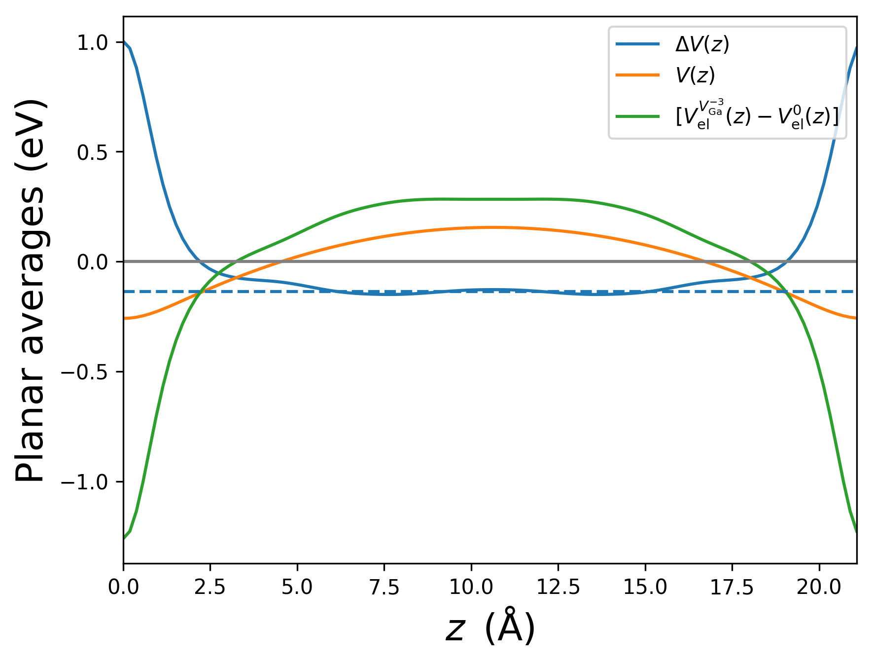
According to the recipe introduced above, we extract the constant \(\Delta V\) from \(\Delta V(z)\) furthest from the defect, corresponding to the middle of the unit cell. The extracted value of \(\Delta V = -0.14\) eV is shown as the dashed line. Note that such a plot provides a consistency check of the FNV scheme; if \(\Delta V(z)\) does not display flat behaviour away from the defect, it is a sign that the model is not describing the true electrostatics sufficiently well.

Taken together, the corrected energy difference is

\[E[V_\mathrm{Ga}^{-3}] - E_0 = [21.78 - (-1.28 ) + (-3)\times(-0.14)] \mathrm{eV} = [21.78 + 1.70] \mathrm{eV} = [23.5] \mathrm{eV}\]

This case is a rather extreme example, since the supercell is rather small and the charge state is large. Nonetheless, the large correction demonstrates the importance of electrostatics.

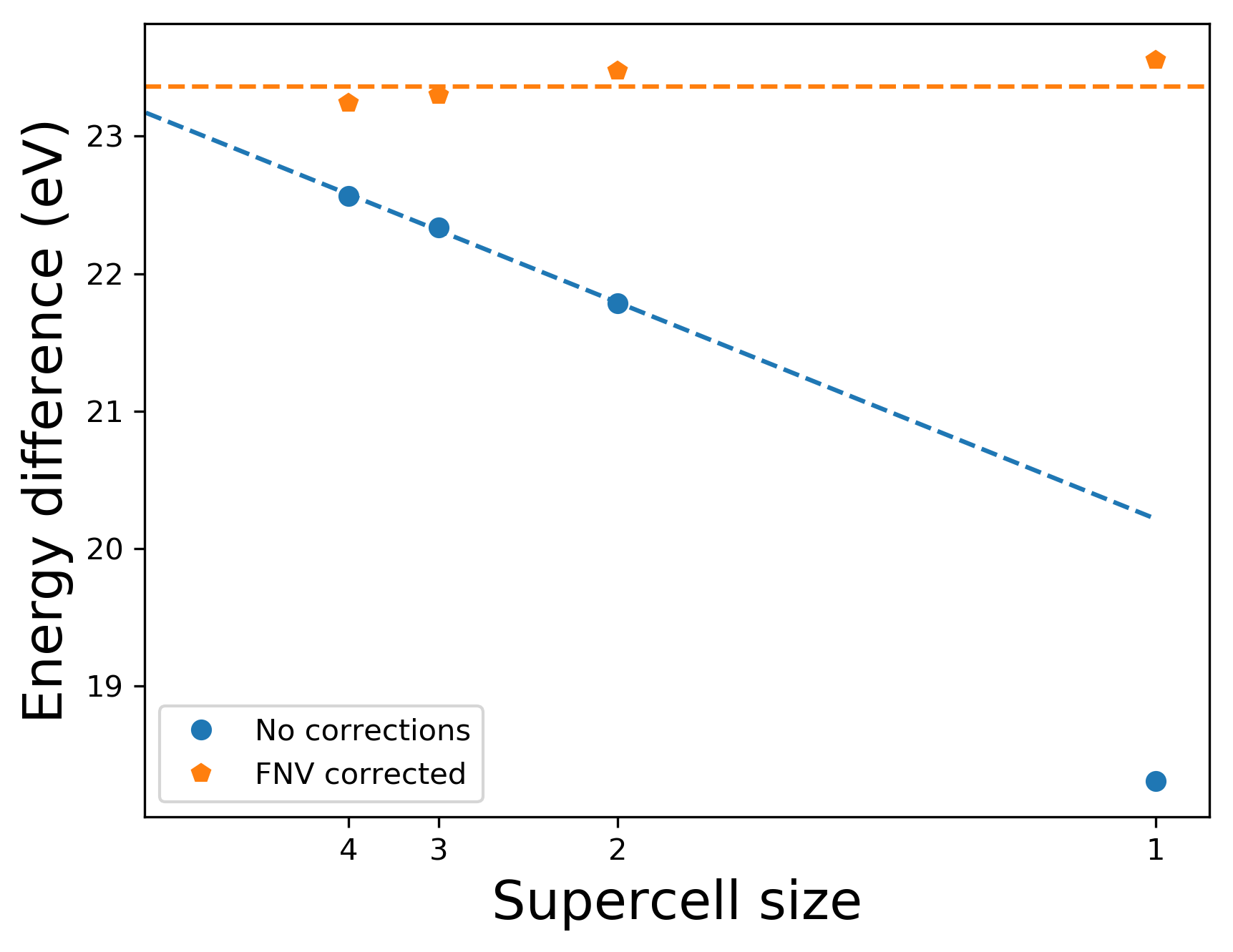
The above calculation can be repeated for different sizes of supercells. The plot below shows the energy differences before and after the FNV corrections are applied, as a function of the number of atoms in the supercell (c.f. Fig. 5 of [3]). The corrections nicely remove the slow convergence due to the electrostatics. Note also that even for the largest supercell (4x4x4, 512 atoms), the electrostatic correction is still large, 0.7 eV.

Additional remarks on calculating formation energies

Here we briefly discuss the other ingredients needed to calculate defect formation energies using the Zhang-Northrup formula. First, the valence band position \(\epsilon_v\) must be obtained from a calculation on the pristine unit cell, with a dense enough \(k\)-point sampling so that the band edge is included (for GaAs this just means that the \(\Gamma\) point is included). Because GPAW always sets the average electrostatic potential to zero, this value is already aligned to the supercell calculation of the pristine sample so needs no further adjustment.

The chemical potentials \(\mu_i\) can be varied, but only within certain limits. For the gallium vacancy we require a value of \(\mu_\mathrm{Ga} \equiv \mu_\mathrm{Ga}[\mathrm{GaAs}]\) , which lies within the range [1]:

\[\mu_\mathrm{Ga}[\mathrm{bulk \ Ga}] > \mu_\mathrm{Ga}[\mathrm{GaAs}]> \mu_\mathrm{Ga}[\mathrm{bulk \ Ga}] + \Delta H_\mathrm{f}[\mathrm{GaAs}]\]

Here, \(\Delta H_\mathrm{f}\) is the enthalpy of formation, and \(\mu_\mathrm{Ga}[\mathrm{bulk \ Ga}]\) the chemical potential corresponding to equilibrium with bulk gallium. Normally one would consider the two limits \(\mu_\mathrm{Ga}[\mathrm{GaAs}] = \mu_\mathrm{Ga}[\mathrm{bulk \ Ga}]\) (“Ga rich”) and \(\mu_\mathrm{Ga}[\mathrm{GaAs}] = \mu_\mathrm{Ga}[\mathrm{bulk \ Ga}] + \Delta H_\mathrm{f}[\mathrm{GaAs}]\) (“As rich”, or “Ga poor”). \(\mu_\mathrm{Ga}[\mathrm{bulk \ Ga}]\) and \(\Delta H_\mathrm{f}[\mathrm{GaAs}]\) can be obtained from total energy calculations on bulk Ga, As, and GaAs.

Carrying out the necessary calculations yields values of 4.75 eV for \(\epsilon_v\) and -3.59 eV for \(\mu_\mathrm{Ga}[\mathrm{bulk \ Ga}]\). Hence the defect formation energy calculated for the 222 cell with and without the FNV corrections, assuming Ga rich conditions, is 5.6 and 3.9 eV respectively (here we also set the position of the electron chemical potential to the top of the valence band, i.e. \(\epsilon_F\) = 0.

Calculation electrostatic corrections in two dimensions

For two-dimensional systems, the approach described above is complicated by the extreme anisotropy of the system, and in particular by the very weak screening occurring between periodically repeated layers. This means that the electrostatic interaction between a localised charge state and its images in neighbouring cells is generally strong, and the corresponding correction is large. The strong interactions pose a number of problems for the correction scheme described above: The heart of the correction scheme is to write the formation energy of the infinitely dilute system as

\[E^f[X^q]_{\infty} = E^f[X^q]_{\mathrm{supercell}} + E_{\mathrm{correction}}.\]

In the limit of an infinitely large supercell, the formation energy in the supercell should approach that of the infinite cell, and the correction should go to zero. To accomplish this in two dimensions, we must be careful about how we scale the cell - If we increase the lateral size of the supercell without changing the vacuum, or if we increase the vacuum without changing the size of the supercell, we get incorrect results. Because of these difficulties, finding a robust correction scheme in 2D is that much more necessary. The starting point is the same as before, and we write:

\[E[X^q] - E_0 = (E[X^q] - E_0)_{\mathrm{uncorrected}} - E_{\mathrm{l}} + q\Delta V.\]

The main problem arises in the \(E_{\mathrm{l}}\) term, and in particular, in finding an appropriate expression for the screened Coulomb interaction of the system.

Recall that \(E_{\mathrm{l}}\) consists of two terms: The energy (per unit cell) associated with the interaction between the model charge distribution and all its periodic images, and the energy of the isolated charge distribution in the same dielectric environment. The first step in calculating either of these is to model the dielectric function.

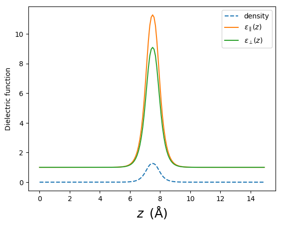
The approach used here is to assume that the dielectric function of the isolated layer is isotropic in plane, and varies only in the \(z\) direction. Additionally, the screening is assumed to follow the density distribution of the system so that we can write

\[\varepsilon_{i}(z) = k_i\cdot n(z) + 1,\]

Where \(i\) varies over “in-plane” and “out-of-plane”, and \(n\) is the in-plane averaged density of the system. The normalization constants, \(k_i\), are chosen such that

\[\begin{split}\frac{1}{L} \int \mathrm{d} z\, \varepsilon_{\parallel}(z) &= \varepsilon_{\parallel}^{\mathrm{DFT}} \\ \frac{1}{L} \int \mathrm{d} z\, \varepsilon_{\perp}^{-1}(z) &= \left(\varepsilon_{\perp}^{\mathrm{DFT}}\right)^{-1}\end{split}\]

The quantities appearing on the right hand side are the in-plane and out-of-plane dielectric constants resulting from a DFT/RPA calculation on the smallest unit cel of the pristine system, but with the same amount of vacuum as the supercell calculation. For 15 Å of vacuum, we calculate \(\varepsilon_{\parallel}^{\mathrm{DFT}} = 1.80\) and \(\varepsilon_{\perp}^{\mathrm{DFT}} = 1.14\). The resulting dielectric profiles are shown below

With the dielectric functions in hand, we can proceed to solve the poisson equation, and calculate the two interaction energies. For more detail on how exactly the potentials and energies of the periodic and isolated charge distributions are calculated, we refer to Localised electrostatic charges in non-uniform dielectric media: Theory.

The following script gives the example of a carbon boron substitution in hexagonal boron nitride:

import sys
import numpy as np
from ase import Atoms
from ase.build import niggli_reduce
from gpaw import GPAW, FermiDirac

# Script to get the total energies of a supercell
# of BN with and without a carbon substitution

c = 15.0

N = int(sys.argv[1])  # NxNx1 supercell
h = 0.15

a = 2.51026699
cell = [[a, 0., 0.],
        [-a / 2, np.sqrt(3) / 2 * a, 0.],
        [0., 0., c]]
scaled_positions = [[2. / 3, 1. / 3, 0.5],
                    [1. / 3, 2. / 3, 0.5]]

system = Atoms('BN',
               cell=cell,
               scaled_positions=scaled_positions,
               pbc=[1, 1, 1])
system = system.repeat((2, 1, 1))
niggli_reduce(system)

defect = system.repeat((N, N, 1))
defect[0].symbol = 'C'
defect[1].magmom = 1

q = +1  # Defect charge

calc = GPAW(mode='fd',
            kpts={'size': (4, 4, 1)},
            xc='PBE',
            charge=q,
            occupations=FermiDirac(0.01),
            txt='BN{0}{0}.CB_charged.txt'.format(N))


defect.calc = calc
defect.get_potential_energy()
calc.write('BN{0}{0}.C_B_charged.gpw'.format(N))

# Neutral case
parameters = calc.todict()
parameters['txt'] = 'BN{0}{0}.CB_neutral.txt'.format(N)
parameters['charge'] = 0
calc = GPAW(**parameters)

defect.calc = calc
defect.get_potential_energy()
calc.write('BN{0}{0}.C_B_neutral.gpw'.format(N))


# Now for the pristine case

pristine = system.repeat((N, N, 1))
parameters['txt'] = 'BN{0}{0}.pristine.txt'.format(N)
calc = GPAW(**parameters)

pristine.calc = calc
pristine.get_potential_energy()
calc.write('BN{0}{0}.pristine.gpw'.format(N))

This script sets up a carbon boron substitution in an NxN supercell of the 4-atom rectangular cell, and calculates the energy of the +1 charge state, the neutral defect and the pristine system, saving the intermediate gpw files.

For the 2x2 system with a vacuum of 15 Å we calculate the uncorrected total energy difference \((E[X^q] - E_0)_\mathrm{uncorrected}\) to be 4.1 eV.

The electrostatic corrections have been implemented in the following script, which greatly resembles the equivalent script for the GaAs defect. The two differences are:

• The dimensionality=2d keyword argument to electrostatic correction constructor, which ensures that the object uses the 2D model for the dielectric functions.

• The use of a list in the set_epsilons() member function, rather than a single number. The first item corresponds to the in-plane dielectric constant, while the second corresponds to the out-of-plane dielectric constant.

import numpy as np
from gpaw.defects import ElectrostaticCorrections
from ase.io import read

sigma = 1.0
q = +1
epsilons = [1.9, 1.15]
corrected = []
uncorrected = []
neutral_energy = []
repeats = [1, 2, 3, 4, 5]
for repeat in repeats:
    pristine = 'BN{0}{0}.pristine.gpw'.format(repeat)
    charged = 'BN{0}{0}.C_B_charged.gpw'.format(repeat)
    neutral = 'BN{0}{0}.C_B_neutral.gpw'.format(repeat)
    elc = ElectrostaticCorrections(pristine=pristine,
                                   charged=charged,
                                   q=q,
                                   sigma=sigma,
                                   dimensionality='2d')
    elc.set_epsilons(epsilons)
    corrected.append(elc.calculate_corrected_formation_energy())
    uncorrected.append(elc.calculate_uncorrected_formation_energy())
    neutral_energy.append(read(neutral).get_potential_energy() -
                          read(pristine).get_potential_energy())
    data = elc.collect_electrostatic_data()
    np.savez('electrostatic_data_BN_{0}{0}.npz'.format(repeat), **data)

np.savez('formation_energies_BN.npz',
         repeats=np.array(repeats),
         corrected=np.array(corrected),
         uncorrected=np.array(uncorrected),
         neutral_energy=np.array(neutral_energy))

As before, we can calculate the formation energy of the charged defect as a function of the supercell size, both with and without the electrostatic corrections. Since all of these systems have the same amount of vacuum, it is not expected that the uncorrected values converge to the true result, but it is encouraging to see the behaviour of the corrected values. As we are dealing with an unrelaxed system, we expect the formation energy of the defect to be too high, but again, the focus is on the electrostatics and the qualitative behaviour as a function of the supercell size, rather than the true values.

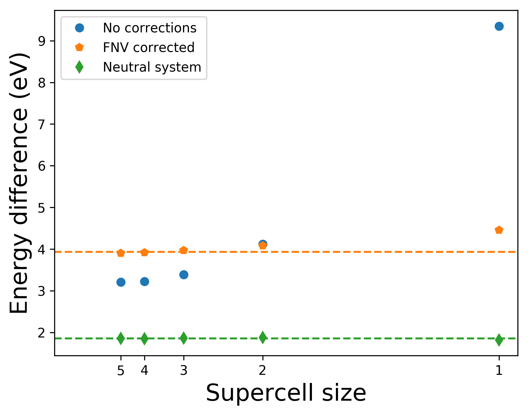
As a test of the quality of the electrostatic corrections, we can look at the charge transition level between the neutral state and the +1 state. This is the energy with respect to the valence band at which the two formation energies are equal, and can be calculated just as \(E_f[X^0] - E_f[X^{+1}]\). It comes to 2 eV, in good agreement with [5].

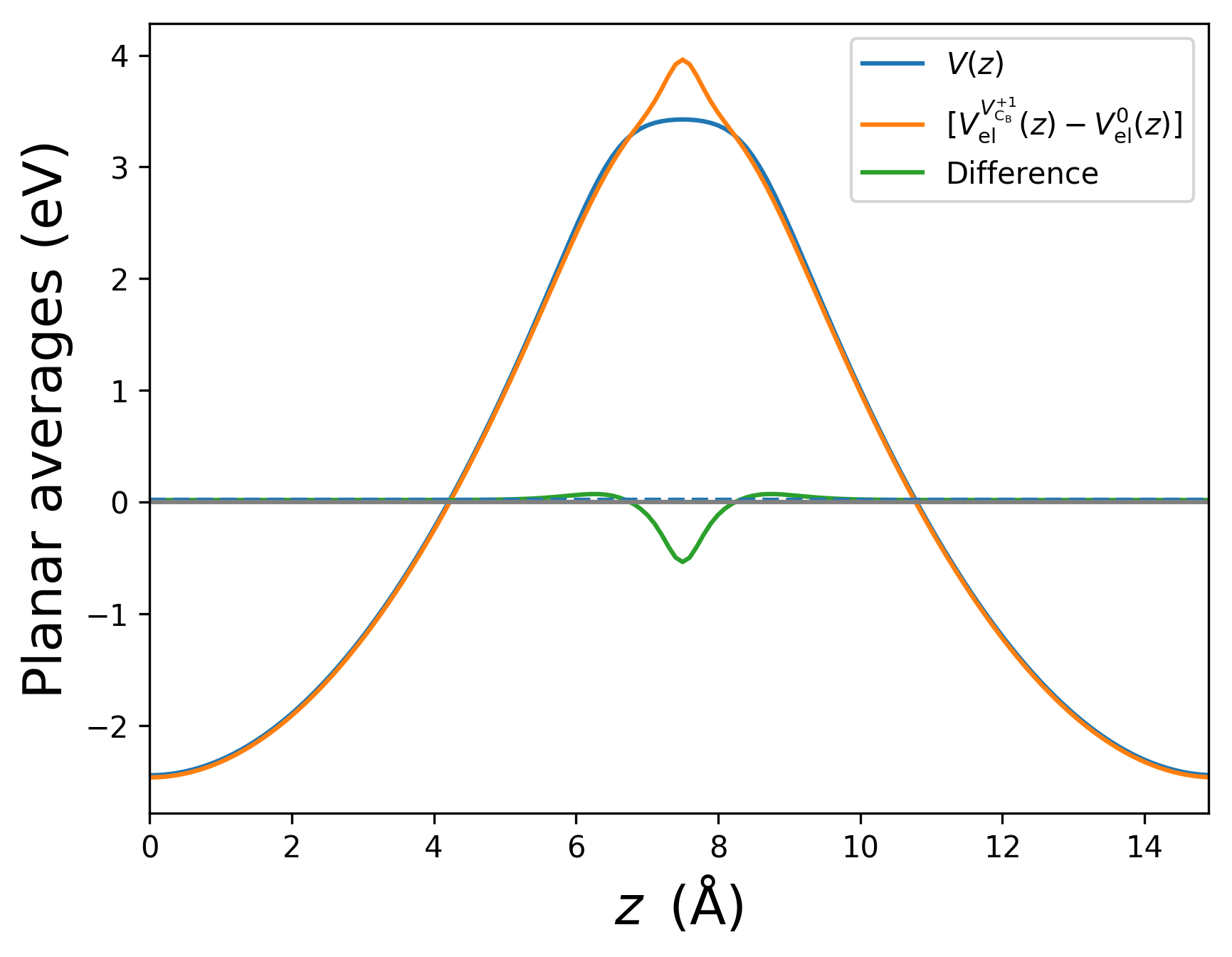
Here are the planar averages (from plot_potentials_BN.py):

References

[1] (1,2)

C. Freysoldt et al. Rev. Mod. Phys. 86, 253 (2014)

[2]

S. Lany and A. Zunger Phys. Rev. B 78, 235104 (2008)

[3] (1,2,3,4)

C. Freysoldt, J. Neugebauer and C. G. Van de Walle Phys. Status Solidi B 248, 1067 (2011)

[4]

H.-P. Komsa, T. T. Rantala and A. Pasquarello Phys. Rev. B 86, 045112 (2012)

[5]

H.-P. Komsa, N. Berseneva, A. V. Krasheninnikov and R. M. Nieminen Phys Rev X 4, 031044 (2014)