Electron transport¶

This exercise shows how to use the ase transport module for performing electron transport calculations in nanoscale contacts.

TransportCalculator is used to calculate transmission functions at two different levels, namely:

Tight-binding (TB) description: parametrize the system using tight-binding model.
DFT description: extract realistic description of the system using the GPAW DFT-LCAO mode.

First-time users of the ASE transport module, should start by reading the methodology in the ASE manual.

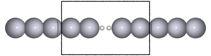
Recent experiments suggests that a hydrogen molecule trapped between metal electrodes has a conductance close to the quantum unit of conductance (\(1G_0=2e^2/h\)). As a manageable model for this system, we consider a hydrogen molecule sandwiched between semi-infinite one dimensional Pt leads as shown in the figure below

… setup …

This is the system considered in the rest of the exercise.

Tight-binding description¶

In this part of the exercise, we illustrate the use of the ASE transport module, by means of a simple tight-binding (TB) model for the Pt-H2-Pt system, with only one TB site per atom. The script can be found here: pt_h2_tb_transport.py. Below we will walk through the script.

As explained in the ASE manual, we need need to define a principal layer, and a scattering region. To be able to describe second nearest neighbor hopping, we choose a principal layer of two Pt atoms. The scattering region is chosen minimal: i.e. the molecule plus one principal layer on each side, as marked with a square on the figure above.

To describe both the principal layer and the coupling between such layers (which is also the coupling from the leads into the scattering region), we define a lead Hamiltonian consisting of two principal layers + coupling:

\[\begin{split}H_\text{lead} = \begin{pmatrix} H_L & V \\ V^\dagger & H_{L} \end{pmatrix}\end{split}\]

Assuming an onsite energy equal to the fermi energy, a nearest neighbor hopping energy of -1, and second nearest neighbor hopping of 0.2, the lead Hamiltonian may be constructed like this:

import numpy as np
H_lead = np.array([[ 0. , -1. ,  0.2,  0. ],
                   [-1. ,  0. , -1. ,  0.2],
                   [ 0.2, -1. ,  0. , -1. ],
                   [ 0. ,  0.2, -1. ,  0. ]])

Next, the Hamiltonian for the scattering region should be constructed. Assuming the Hydrogen molecule can be described by the Hamiltonian:

\[\begin{split}H_\text{mol} = \begin{pmatrix} 0 & -0.8 \\ -0.8 & 0 \end{pmatrix}\end{split}\]

and that the molecule only couples to the nearest Pt atom, with a hopping energy of 0.2: Write down the explicit scattering Hamiltonian (it is a \(6 \times 6\) matrix).

You are now ready to initialize the TransportCalculator:

from ase.transport.calculators import TransportCalculator

tcalc = TransportCalculator(h=H_scat,  # Scattering Hamiltonian
                            h1=H_lead, # Lead 1 (left)
                            h2=H_lead, # Lead 2 (right)
                            pl=2)      # principal layer size

To calculate the transmission function; first select an energy grid for the transmission, then run tcalc.get_transmission():

tcalc.set(energies=py.arange(-3, 3, 0.02))
T_e = tcalc.get_transmission()

Try to plot the transmission function (e.g. using pylab.plot(tcalc.energies, T_e)).

The projected density of states (pdos) for the two hydrogen TB sites can be calculated using:

tcalc.set(pdos=[0, 1])
pdos_ne = tcalc.get_pdos()

Note that all indices in TransportCalculator refers to the scattering region minus the mandatory principal layer on each side. Why do you think the pdos of each the hydrogen TB sites has two peaks?

To investigate the system you can try to diagonalize the subspace spanned by the hydrogen TB sites:

h_rot, s_rot, eps_n, vec_nn = tcalc.subdiagonalize_bfs([0, 1])
tcalc.set(h=h_rot, s=s_rot) # Set the rotated matrices

eps_n[i] and vec_nn[:,i] contains the i’th eigenvalue and eigenvector of the hydrogen molecule. Try to calculate the pdos again. What happpened?

You can try to remove the coupling to the bonding state and calculate the calculate the transmission function:

tcalc.cutcupling_bfs([0])
T_cut_bonding_e = tcalc.get_transmission()

You may now understand the transport behavior of the simple model system. The transmission peak at -0.8 eV and 0.8 eV are due to the bonding and antibonding states of the TB described hydrogen molecule.

DFT description¶

We now continue to explore the Pt-H2-Pt system using a more realistic desciption derived from ab-initio calculations.

The functions gpaw.lcao.tools.get_lcao_hamiltonian and gpaw.lcao.tools.get_lead_lcao_hamiltonian (in gpaw.lcao.tools) allows you to construct such a Hamiltonian within DFT in terms of pseudo atomic orbitals. Since real potential decay much slower than in our TB model, we increase the principal layers to 4 Pt atoms, and the scattering region to 5 Pt atoms on either side. To obtain the matrices for the scattering region and the leads using DFT and pseudo atomic orbitals using a szp basis set run this pt_h2_lcao_manual.py:

#!/usr/bin/env python
"""Transport exersice

This file should do the same as pt_h2_lcao.py, but extracts the Hamiltonians
manually instead of using gpawtransport, which currently does not work
"""

from ase import Atoms
from gpaw import GPAW, Mixer, FermiDirac
from gpaw.lcao.tools import (remove_pbc,
                             get_lcao_hamiltonian,
                             get_lead_lcao_hamiltonian)
import pickle as pickle

a = 2.41  # Pt binding length
b = 0.90  # H2 binding length
c = 1.70  # Pt-H binding length
L = 7.00  # width of unit cell

#####################
# Scattering region #
#####################

# Setup the Atoms for the scattering region.
atoms = Atoms('Pt5H2Pt5', pbc=(1, 0, 0), cell=[9 * a + b + 2 * c, L, L])
atoms.positions[:5, 0] = [i * a for i in range(5)]
atoms.positions[-5:, 0] = [i * a + b + 2 * c for i in range(4, 9)]
atoms.positions[5:7, 0] = [4 * a + c, 4 * a + c + b]
atoms.positions[:, 1:] = L / 2.

# Attach a GPAW calculator
calc = GPAW(h=0.3,
            xc='PBE',
            basis='szp(dzp)',
            occupations=FermiDirac(width=0.1),
            kpts=(1, 1, 1),
            mode='lcao',
            txt='pt_h2_lcao_scat.txt',
            mixer=Mixer(0.1, 5, weight=100.0),
            symmetry={'point_group': False, 'time_reversal': False})
atoms.calc = calc

atoms.get_potential_energy()  # Converge everything!
Ef = atoms.calc.get_fermi_level()

H_skMM, S_kMM = get_lcao_hamiltonian(calc)
# Only use first kpt, spin, as there are no more
H, S = H_skMM[0, 0], S_kMM[0]
H -= Ef * S
remove_pbc(atoms, H, S, 0)

# Dump the Hamiltonian and Scattering matrix to a pickle file
pickle.dump((H.astype(complex), S.astype(complex)),
            open('scat_hs.pickle', 'wb'), 2)

########################
# Left principal layer #
########################

# Use four Pt atoms in the lead, so only take those from before
atoms = atoms[:4].copy()
atoms.set_cell([4 * a, L, L])

# Attach a GPAW calculator
calc = GPAW(h=0.3,
            xc='PBE',
            basis='szp(dzp)',
            occupations=FermiDirac(width=0.1),
            kpts=(4, 1, 1),  # More kpts needed as the x-direction is shorter
            mode='lcao',
            txt='pt_h2_lcao_llead.txt',
            mixer=Mixer(0.1, 5, weight=100.0),
            symmetry={'point_group': False, 'time_reversal': False})
atoms.calc = calc

atoms.get_potential_energy()  # Converge everything!
Ef = atoms.calc.get_fermi_level()

ibz2d_k, weight2d_k, H_skMM, S_kMM = get_lead_lcao_hamiltonian(calc)
# Only use first kpt, spin, as there are no more
H, S = H_skMM[0, 0], S_kMM[0]
H -= Ef * S

# Dump the Hamiltonian and Scattering matrix to a pickle file
pickle.dump((H, S), open('lead1_hs.pickle', 'wb'), 2)

#########################
# Right principal layer #
#########################
# This is identical to the left prinicpal layer so we don't have to do anything
# Just dump the same Hamiltonian and Scattering matrix to a pickle file
pickle.dump((H, S), open('lead2_hs.pickle', 'wb'), 2)

You should now have the files scat_hs.pickle, lead1_hs.pickle and lead2_hs.pickle in your directory.

You are now ready to initialize the TransportCalculator: The script can be found here: pt_h2_lcao_transport.py. Below we will work through the script.

The pickle files can be loaded and used in the TransportCalculator:

from ase.transport.calculators import TransportCalculator
import pickle

#Read in the hamiltonians
h, s = pickle.load(open('scat_hs.pickle', 'rb'))
h1, s1 = pickle.load(open('lead1_hs.pickle', 'rb'))
h2, s2 = pickle.load(open('lead2_hs.pickle', 'rb'))

tcalc = TransportCalculator(h=h, h1=h1, h2=h2, # hamiltonian matrices
                            s=s, s1=s1, s2=s2, # overlap matrices
                            align_bf=1)        # align the Fermi levels

In SZP there are 4 basis functions per H atom, and 9 per Pt atom. Does the size of the different matrices match your expectations? What is the conductance? Does it agree with the experimental value?

We will now try to investigate transport properties in more detail. Try to subdiagonalize the molecular subspace:

Pt_N = 5
Pt_nbf = 9 # number of bf per Pt atom (basis=szp)
H_nbf = 4  # number of bf per H atom (basis=szp)
bf_H1 = Pt_nbf * Pt_N
bfs = range(bf_H1, bf_H1 + 2 * H_nbf)
h_rot, s_rot, eps_n, vec_jn = tcalc.subdiagonalize_bfs(bfs)
for n in range(len(eps_n)):
    print('bf %i correpsonds to the eigenvalue %.2f eV' % (bfs[n],eps_n[n]))

Argue that vec_jn[:,0] and vec_jn[:,1] corresponds to the bonding and anti-bonding molecular hydrogen orbitals, respectively.

What is the calculated band-gap of the hydrogen-molecule?

Switch to the rotated basis set (tcalc.set(h=h_rot, s=s_rot)) then plot the transmission function end the projected density of states of the renormalized molecular orbitals in an energy range of say -8 to 4 eV.

Which orbital do you think is responsible for the high conductance? Try to cut the relevant orbitals from the basis set, as we did for the TB model.

The TransportCalculator class¶

class ase.transport.calculators.TransportCalculator(**kwargs)[source]¶

Determine transport properties of a device sandwiched between two semi-infinite leads using a Green function method.

Create the transport calculator.

Parameters:

h(N, N) ndarray: Hamiltonian matrix for the central region.
s{None, (N, N) ndarray}, optional: Overlap matrix for the central region. Use None for an orthonormal basis.
h1(N1, N1) ndarray: Hamiltonian matrix for lead1.
h2{None, (N2, N2) ndarray}, optional: Hamiltonian matrix for lead2. You may use None if lead1 and lead2 are identical.
s1{None, (N1, N1) ndarray}, optional: Overlap matrix for lead1. Use None for an orthonomormal basis.
hc1{None, (N1, N) ndarray}, optional: Hamiltonian coupling matrix between the first principal layer in lead1 and the central region.
hc2{None, (N2, N} ndarray), optional: Hamiltonian coupling matrix between the first principal layer in lead2 and the central region.
sc1{None, (N1, N) ndarray}, optional: Overlap coupling matrix between the first principal layer in lead1 and the central region.
sc2{None, (N2, N) ndarray}, optional: Overlap coupling matrix between the first principal layer in lead2 and the central region.
energies{None, array_like}, optional: Energy points for which calculated transport properties are evaluated.
eta{1.0e-5, float}, optional: Infinitesimal for the central region Green function.
eta1/eta2{1.0e-5, float}, optional: Infinitesimal for lead1/lead2 Green function.
align_bf{None, int}, optional: Use align_bf=m to shift the central region by a constant potential such that the m’th onsite element in the central region is aligned to the m’th onsite element in lead1 principal layer.
logfile{None, str}, optional: Write a logfile to file with name \(logfile\). Use ‘-’ to write to std out.
eigenchannels: {0, int}, optional: Number of eigenchannel transmission coefficients to calculate.
pdos{None, (N,) array_like}, optional: Specify which basis functions to calculate the projected density of states for.
dos{False, bool}, optional: The total density of states of the central region.
box: XXX: YYY

If hc1/hc2 are None, they are assumed to be identical to the coupling matrix elements between neareste neighbor principal layers in lead1/lead2.

Examples:

>>> import numpy as np
>>> h = np.array((0,)).reshape((1,1))
>>> h1 = np.array((0, -1, -1, 0)).reshape(2,2)
>>> energies = np.arange(-3, 3, 0.1)
>>> calc = TransportCalculator(h=h, h1=h1, energies=energies)
>>> T = calc.get_transmission()