(Resonant-)Raman spectra of gas-phase water
This tutorial shows how to calculate (resonant-)Raman spectra of a single water molecule in the gas-phase. The theoretical background can be found in Ref. [1].
Accurate Forces from an IR calculation
A pre-condition for accurate forces and thus accurate vibrational frequencies
is relaxation with a rather small maximal force and a smaller gid-spacing
than is needed for excitated state calculations.
This is possible using the Vibrations or
Infrared
modules.
from ase import optimize
from ase.build import molecule
from ase.vibrations.infrared import Infrared
from gpaw import GPAW, FermiDirac
from gpaw.cluster import Cluster

h = 0.20

atoms = Cluster(molecule('H2O'))
atoms.minimal_box(4, h=h)

# relax the molecule
calc = GPAW(mode='fd', xc='PBE', h=h, occupations=FermiDirac(width=0.1))
atoms.calc = calc

dyn = optimize.FIRE(atoms)
dyn.run(fmax=0.01)
atoms.write('relaxed.traj')

# finite displacement for vibrations
atoms.calc = calc.new(symmetry={'point_group': False})
ir = Infrared(atoms, name='ir')
ir.run()
We can get the resulting frequencies
# web-page: H2O_ir_summary.txt
from ase import io
from ase.vibrations.infrared import Infrared

atoms = io.read('relaxed.traj')
ir = Infrared(atoms, name='ir')
with open('H2O_ir_summary.txt', 'w') as fd:
    ir.summary(log=fd)
with the result:
-------------------------------------
 Mode    Frequency        Intensity
  #    meV     cm^-1   (D/Å)^2 amu^-1
-------------------------------------
  0   27.6i    222.9i     0.0191
  1   24.1i    194.1i     0.5781
  2   20.7i    167.0i     4.5786
  3   19.5i    157.4i     0.1154
  4   16.4i    132.5i     0.0028
  5   29.7     239.9      1.8390
  6  198.7    1602.7      1.6508
  7  461.5    3722.0      0.0679
  8  474.3    3825.4      1.2356
-------------------------------------
Zero-point energy: 0.582 eV
Static dipole moment: 1.825 D
Maximum force on atom in `equilibrium`: 0.0094 eV/Å
Only the last three vibrations are meaningful.
Static Raman from polarizabilities
The photon energy of the excitation laser in Raman experiments is often well below electronic excitations of the molecules. Then the approximation to obtain Raman spectra from static polarizabilities is valid. Here, we use the static polariability obtained from external electric fields.
from ase.vibrations.raman import StaticRamanCalculator
from gpaw import GPAW, FermiDirac
from gpaw.cluster import Cluster
from gpaw.external import static_polarizability


h = 0.2
xc = 'PBE'
atoms = Cluster('relaxed.traj')
atoms.minimal_box(4., h=h)

atoms.calc = GPAW(mode='fd', xc=xc, h=h,
                  occupations=FermiDirac(width=0.1),
                  symmetry={'point_group': False})
atoms.get_potential_energy()


class Polarizability:
    def __call__(self, atoms):
        return static_polarizability(atoms)


name = exname = 'static_raman'
ram = StaticRamanCalculator(
    atoms, Polarizability, name=name)
ram.run()

ram.summary()
We can get the resulting frequencies and intensities
# web-page: H2O_Placzek_static_summary.txt
from ase import io
from ase.vibrations.placzek import PlaczekStatic

atoms = io.read('relaxed.traj')
ram = PlaczekStatic(atoms, name='static_raman')
with open('H2O_Placzek_static_summary.txt', 'w') as fd:
    ram.summary(log=fd)
with the result:
-------------------------------------
 Mode    Frequency        Intensity
  #    meV     cm^-1      [A^4/amu]
-------------------------------------
  0    0.0       0.0        0.00
  1    0.0       0.0        0.00
  2    0.0       0.0        0.00
  3    0.0       0.0        0.00
  4    0.0       0.0        0.02
  5   32.2     260.1        0.00
  6  199.1    1605.6        0.87
  7  461.3    3720.5      112.74
  8  474.1    3823.9       27.21
-------------------------------------
Again, only the last three vibrations are meaningful.
Resonant Raman: Excitations at each displacement
We need to calculate the excitations at each displament and use
linear response TDDFT for this. This is the most time consuming
part of the calculation an we therfore use the coarser grid spacing
of h=0.25. We restrict to the first excitations
of the water molecule by setting
{'restrict': {'energy_range': erange, 'eps': 0.4}}.
Note, that the number of bands in the calculation is connected
to this.
from ase.vibrations.resonant_raman import ResonantRamanCalculator
from gpaw import GPAW, FermiDirac
from gpaw.cluster import Cluster
from gpaw.lrtddft import LrTDDFT

h = 0.25
xc = 'PBE'
atoms = Cluster('relaxed.traj')
atoms.minimal_box(4., h=h)

atoms.calc = GPAW(mode='fd', xc=xc, h=h, nbands=50,
                  occupations=FermiDirac(width=0.1),
                  eigensolver='cg', symmetry={'point_group': False},
                  convergence={'eigenstates': 1.e-5, 'bands': -10})
atoms.get_potential_energy()

erange = 17
ext = '_erange{0}'.format(erange)
gsname = exname = 'rraman' + ext
rr = ResonantRamanCalculator(
    atoms, LrTDDFT, name=gsname, exname=exname,
    exkwargs={'restrict': {'energy_range': erange, 'eps': 0.4}},)
rr.run()
Raman intensities
We have to choose an approximation to evaluate the Raman intensities.
The most common is the Placzek approximation which we also apply here.
We may use summary() similar to Infrared,
but the Raman intensity depends on the excitation frequency.
# web-page: H2O_rraman_summary.txt
from ase import io
from ase.vibrations.placzek import Placzek
from gpaw.lrtddft import LrTDDFT

atoms = io.read('relaxed.traj')
pz = Placzek(atoms, LrTDDFT,
             name='ir',  # use ir-calculation for frequencies
             exname='rraman_erange17')  # use LrTDDFT for intensities

omega = 0  # excitation frequency
gamma = 0.2  # width
with open('H2O_rraman_summary.txt', 'w') as fd:
    pz.summary(omega, gamma, log=fd)
with the result:
-------------------------------------
 excitation at 0 eV
 gamma 0.2 eV
 method: standard
 approximation: PlaczekAlpha
 Mode    Frequency        Intensity
  #    meV     cm^-1      [A^4/amu]
-------------------------------------
  0    0.0       0.0        0.01
  1    0.0       0.0        0.00
  2    0.0       0.0        0.01
  3    0.0       0.0        0.41
  4    0.0       0.0        1.12
  5   29.7     239.9        0.12
  6  198.7    1602.7       43.34
  7  461.5    3722.0      154.80
  8  474.3    3825.4       57.13
-------------------------------------
Zero-point energy: 0.582 eV
Note, that the absolute intensity [1] is given in the summary.
Raman spectrum
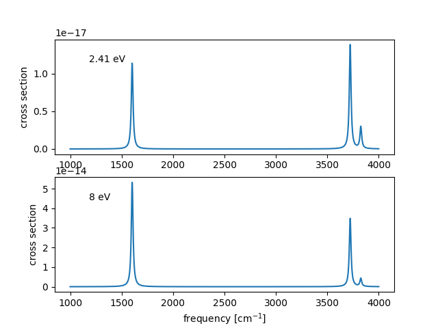
The Raman spectrum be compared to experiment shown above can be obtained with the following script
# web-page: H2O_rraman_spectrum.png
import matplotlib.pyplot as plt
from ase import io
from ase.vibrations.placzek import Placzek
from gpaw.lrtddft import LrTDDFT

atoms = io.read('relaxed.traj')
pz = Placzek(atoms, LrTDDFT,
             name='ir',  # use ir-calculation for frequencies
             exname='rraman_erange17')  # use LrTDDFT for intensities

gamma = 0.2  # width

for i, omega in enumerate([2.41, 8]):  # photon energies
    plt.subplot(211 + i)
    x, y = pz.get_spectrum(omega, gamma,
                           start=1000, end=4000, type='Lorentzian')
    plt.text(0.1, 0.8, f'{omega} eV', transform=plt.gca().transAxes)
    plt.plot(x, y)
    plt.ylabel('cross section')

plt.xlabel('frequency [cm$^{-1}$]')
plt.savefig('H2O_rraman_spectrum.png')
The figure shows the sensitivity of relative peak heights on the scattered photons energy.