Raman spectroscopy for extended systems

This tutorial shows how to calculate the Raman spectrum of bulk MoS_2 (MoS2_2H_relaxed_PBE.json) using the electron-phonon coupling based Raman methods as described in Raman spectroscopy.

Effective Potential

At the heart of the electron-phonon coupling is the calculation of the gradient of the effective potential, which is done using finite displacements just like the phonons. Those two calculations can run simultaneous, of the required set of parameters coincide.

The electron-phonon matrix is quite sensitive to self-interaction of a displaced atom with its periodic images, so a sufficiently large supercell needs to be used. The (3x3x2) supercell used in this example should be barely enough. When using a supercell for the calculation you have to consider, that the atoms object needs to contain the primitive cell, not the supercell, while the parameters for the calculator object need to be good for the supercell, not the primitive cell. (displacement.py)

from ase.io import read
from gpaw import GPAW, FermiDirac, PW
from gpaw.elph import DisplacementRunner


def get_pw_calc(ecut, kpts):
    return GPAW(mode=PW(ecut),
                parallel={'sl_auto': True, 'augment_grids': True},
                xc='PBE',
                kpts=kpts,
                occupations=FermiDirac(0.02),
                convergence={'energy': 1e-6,
                             'density': 1e-6},
                symmetry={'point_group': False},
                txt='displacement.txt')


atoms = read("MoS2_2H_relaxed_PBE.json")
calc = get_pw_calc(700, (2, 2, 2))
elph = DisplacementRunner(atoms=atoms, calc=calc,
                          supercell=(3, 3, 2), name='elph',
                          calculate_forces=True)
elph.run()

This calculation merely dumped the effective potential at various displacements onto the harddrive. We now need to calculate the actual derivative and project them onto a set of LCAO basis functions.

For this we first need to complete a ground-state calculation for the supercell. This calculation needs to be done in LCAO mode with parallelisation over domains and bands disabled. (supercell.py)

from ase.io import read
from gpaw import GPAW, FermiDirac
from gpaw.elph import Supercell


def get_lcao_calc(gpt, kpts):
    return GPAW(mode='lcao',
                parallel={'sl_auto': True, 'augment_grids': True,
                          'domain': 1, 'band': 1},
                xc='PBE',
                gpts=gpt,
                kpts=kpts,
                occupations=FermiDirac(0.02),
                symmetry={'point_group': False},
                txt='supercell.txt')


atoms = read("MoS2_2H_relaxed_PBE.json")
atoms_N = atoms * (3, 3, 2)
calc = get_lcao_calc((60, 60, 160), (2, 2, 2))

atoms_N.calc = calc
atoms_N.get_potential_energy()

sc = Supercell(atoms=atoms, supercell=(3, 3, 2))
sc.calculate_supercell_matrix(calc, fd_name='elph')

The calculate_supercell_matrix() method will then compute the gradients and calculate the matrix elements. The results are saved in a file cache in a basis of LCAO orbitals and supercell indices.

If you use the planewave mode for the displacement calculation, please see the note in Electron-phonon coupling.

Phonons

The phonon frequencies enter the Raman calculation by defining the line positions in the final spectrum. Their associated mode vectors are necessary to project the electron-phonon matrix from Cartesian coordinates in the modes.

It is crucial to use tightly relaxed structures and well-converged parameters to obtain accurate phonon frequencies. We already calculated the forces in the previous step and need only the extract the phonon frequencies for later usage. (phonons.py)

# Phonon calculation
ph = Phonons(atoms, supercell=(3, 3, 2), name="elph", center_refcell=True)

ph.read(method='frederiksen', acoustic=True, )
frequencies = ph.band_structure([[0, 0, 0], ])[0]  # Get frequencies at Gamma

# save phonon frequencies for later use
np.save("vib_frequencies.npy", frequencies)

As exercise, check the dependence of the phonon frequencies with the calculation mode, supercell size and convergence parameters.

This given set of parameters yield this result:

  i    cm^-1
------------
  0   -11.21
  1    -2.75
  2     3.20
  3    29.01
  4    29.57
  5    55.19
  6   276.02
  7   276.44
  8   277.94
  9   278.39
 10   370.99
 11   371.43
 12   371.69
 13   371.95
 14   399.12
 15   402.67
 16   456.72
 17   460.57

Momentum matrix

The Raman tensor does not only depend on the electron-phonon matrix, but also on the transition probability between electronic states, which in this case is expressed in the momentum matrix elements. Those can be extracted directly from a converged LCAO calculation (scf.py) of the primitive cell. (dipolemoment.py)

from gpaw import GPAW
from gpaw.lcao.dipoletransition import get_momentum_transitions


calc = GPAW("scf.gpw")

if not hasattr(calc.wfs, 'C_nM'):
    print("Need to initialise")
    calc.initialize_positions(calc.atoms)
get_momentum_transitions(calc.wfs, savetofile=True)

Phonon mode projected electron-phonon matrix

With all the above calculations finished we can extract the electron-phonon matrix in the Bloch basis of the primitive cell projected onto the phonon modes: (gmatrix.py)

from gpaw import GPAW
from gpaw.elph import ElectronPhononMatrix

calc = GPAW("scf.gpw")
atoms = calc.atoms

elph = ElectronPhononMatrix(atoms, 'supercell', 'elph')
q = [[0., 0., 0.], ]
g_sqklnn = elph.bloch_matrix(calc, k_qc=q,
                             savetofile=True, prefactor=False)

This will save the electron-phonon matrix as a numpy file to the disk. The optional load_sc_as_needed tag prevents from all supercell cache files being read at once. Instead they are loaded and processed one-by-one. This can save lots of memory for larger systems with hundreds of atoms, where the supercell matrix can be over 100GiB large.

Note: This part has not been tested properly for parallel runs and should be done in serial mode only.

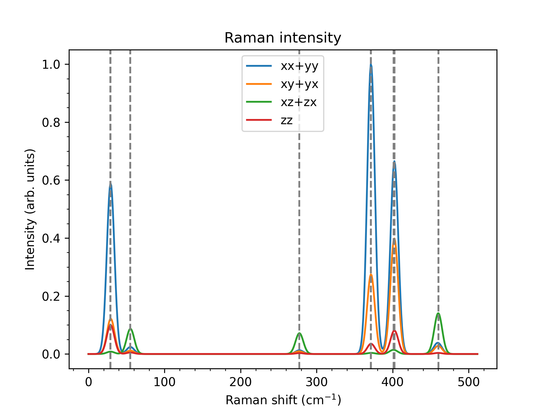
Raman spectrum

With all ingredients provided we can now commence with the computation of the Raman tensor which is saved in a file cache.(raman.py)

import numpy as np

from gpaw.calculator import GPAW
from gpaw.elph import ResonantRamanCalculator


calc = GPAW("scf.gpw", parallel={'domain': 1, 'band': 1})
wph_w = np.load("vib_frequencies.npy")

rrc = ResonantRamanCalculator(calc, wph_w)
rrc.calculate_raman_tensor(rrc.nm_to_eV(488.))

The final result can then be plotted:(plot_spectrum.py)

from gpaw.elph import RamanData

rd = RamanData()
entries = [["xx", "yy"], ["xy", "yx"], ["xz", "zx"], ["zz", ]]

spectra = []
labels = []
for entry in entries:
    energy, spectrum = rd.calculate_raman_spectrum(entry)
    spectra.append(spectrum)
    if len(entry) == 2:
        label = entry[0] + "+" + entry[1]
    else:
        label = entry[0]
    labels.append(label)

rd.plot_raman("Polarised_raman_488nm.png", energy, spectra, labels,
              relative=False)