Solvated Jellium (constant-potential electrochemistry)

Overview

The Solvated Jellium method (SJM) is a simple method for the simulation of electrochemical interfaces in DFT. A full description of the approach can be found in [Kastlunger2018]. The method allows you to control the simulated electrode potential (manifested as the topside work function) by varying the number of electrons in the simulation; calculations can be run in either constant-charge or constant-potential mode. The SJM calculator can be used just like the standard GPAW calculator; it returns energy and forces, but can do so at a fixed potential. (Please see the note below on the Legendre-transform of the energy.) The potential is controlled by a simple iterative technique; in practice if you are running a trajectory (such as a relaxation or nudged elastic band) the first image will take longer than a conventional calculation as the potential equilibrates, but the computational cost is much less on subsequent images; practically, we estimate the extra cost to be <50% compared to a traditional DFT calculation of a full trajectory. For a practical guide on the use of the method, please see the Solvated Jellium Method (SJM) tutorial.

Theoretical background

The philosophy of the solvated jellium method is to construct the simplest model that captures the physics of interest, without introducing spurious effects. The solvated jellium approach consists of two components: jellium and an implicit solvent. A schematic is shown below:

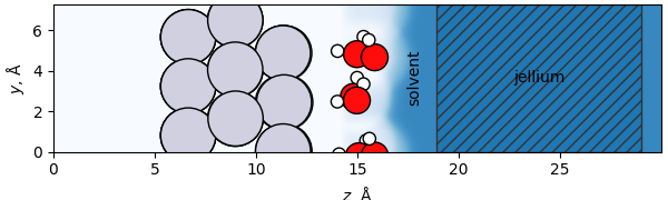
In this figure, the jellium is shown by the hashed marks, while the implicit solvent is shown in the blue shaded region. Note that an explicit solvent (the water molecules) is also conventionally used in this approach, as the major purpose of the implicit solvent is not to simulate the solvation of individual species but rather to screen the net field. A more detailed discussion of both of these components follows.

The jellium slab: charging

In a periodic system we cannot have a net charge; therefore, any additional, fractional electrons that are added to the system must be compensated by an equal amount of counter charge. In GPAW, this is conveniently accomplished with a JelliumSlab. This adds a smeared-out background charge in a fixed region of the simulation cell; in the figure above it is shown as the dashed region to the right of the atoms. The JelliumSlab also increases the number of electrons in the simulation by an amount equal to the total charge of the slab. 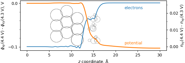When you run a simulation, you should see that these excess electrons localize on the \(+z\) side (the right side in these figures) of the metal atoms that simulate the electrode surface, and not on the \(-z\) (left) side, which simulates the bulk. This is accomplished by only putting the jellium region on one side of the simulation, and employing a dipole correction (included by default when you run SJM) to electrostatically decouple the two sides of the cell.

The figure below shows the difference in two simulations, one run at 4.4 V and one run at 4.3 V. The orange curve shows where the potential drops off, and the blue curve shows where the electrons localize.

The jellium region is conventionally thought of as a region of smeared-out positive charge, accompanied by a positive number of electrons. However, the signs can readily be reversed, making the jellium region a smeared-out negative region accompanied by a reduction in the total number of electrons. In this way, the same tool can be used to perturb the electrons in either a positive or negative direction, and thus vary the potential in either direction in order to find its target. Note also that the jellium region does not overlap any atoms, separating this from approaches that employ a homogeneous background charge throughout the unit cell (in which spurious interactions can occur). This is important to not distort the electronic structure of the atoms and molecules being simulated. Additionally, note that the jellium is enclosed in a regular slab geometry in the figure above, but this need not be the case; it can, for example, follow the cavity of the implicit solvent if this is preferred (by using the jelliumregion keyword as described in the SJM documentation).

The solvation: screening

By itself, the excess electrons and the jellium counter charge would set up an artificially high potential field in the region of the reaction. To screen this large field, an implicit solvent is added to the simulation in the region above the explicit solvent, completely surrounding the jellium counter charge. For this purpose, the solvated jellium method employs the implicit solvation model of Held and Walter [Held2014], which changes the dielectric constant of the vacuum region. (You can learn more about the solvation method in the Continuum Solvent Model (CSM) tutorial.)

Here, the primary purpose of the implicit solvent is not to solvate the species reacting at the surface; explicit solvent (shown by the water molecules above) is typically employed in SJ simulations for this purpose. The implicit solvent is located above the explicit solvent (and therefore may provide some solvent stabilization to the explicit solvent molecules). This can be seen in the figure above, where the implicit solvent is shown as the blue shaded region. In this figure, the small amount of solvent that is apparent at a \(z\) coordinate corresponding to the water layer is just the result of the implicit solvent penetrating slightly into the cavity at the center of a hexagonal ice-like water structure. It is important that the implicit solvent not be present in the region of the reaction, as this would be “double”-solvating those parts. If this occurs, “ghost” atoms can be added to exclude the solvent from specific regions.

Generalized Poisson equation

In net, the SJ method is manifested as two changes to the generalized Poisson equation,

\[\vec{\nabla} \cdot \Big(\epsilon(\br) \vec{\nabla} \phi(\br)\Big) = -4\pi \Big[ \rho_\mathrm{explicit}(\br) + \rho_\mathrm{jellium} (\br) \Big],\]

where \(\epsilon(\br)\) accounts for the solvation; that is, the dielectric constant is spatially variant, and the spatially-resolved charge density is modified by the presence of the \(\rho_\mathrm{jellium}(\br)\) term, which contains the smeared-out counter charge in a region away from all of the atoms (and electronic density) of the system. \(\rho_\mathrm{explicit} (\br)\) contains the standard charge density of the system; that is, due to the electrons and nuclei. Since the changes to the Poisson equation are relatively simple, it can be solved without relying on linearization.

The electrode potential

The electrode potential (\(\phi_\mathrm{e}\)) is then defined as the Fermi-level energy (\(\mu\)) referenced to a point deep in the solvent (\(\Phi_\mathrm{w}\)), where the whole charge on the electrode has been screened and no electric field is present. (This is equivalently the topside work function of the slab.) This is divided by the unit electronic charge \(e\) to convert from energy (typically in eV) to potential (typically in V) dimensions.

\[\phi_\mathrm{e} = \frac{\Phi_\mathrm{w} - \mu}{e} .\]

Note that this gives the potential with respect to vacuum; if you would like your potential on a reference electrode scale, such as SHE, please see the Solvated Jellium Method (SJM) tutorial.

Legendre-transformed energy

The energy used in the analysis of electrode reactions is the grand-potential energy

\[\Omega \equiv E_\mathrm{tot} + N_\mathrm{e}e \phi_\mathrm{e} .\]

Whereas \(E_\mathrm{tot}\) is consistent with the forces in traditional electronic structure calculations, the grand-potential energy \(\Omega\) is consistent with the forces in electronically grand-canonical (that is, constant-potential) simulations. This means that relaxations that follow forces will find local minima in \(\Omega\), and generally methods that rely on consistent force and energy information (such as BFGSLineSearch or NEB) will work fine as long as \(\Omega\) is employed. Thus, this calculator returns \(\Omega\) by default, rather than \(E_\mathrm{tot}\).

Potential control

The below figure shows both the localization of excess electrons and the local change in potential, when the total number of electrons in an example simulation are changed.

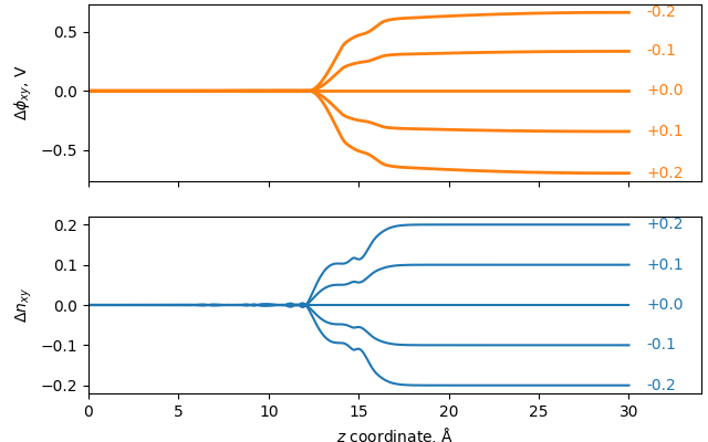
As mentioned above, the excess electrons localize only on the top side of the slab, which is meant to represent the electrode surface, and not on the bottom side, which is mean to represent the bulk. The potential drop is seen to localize in the Stern layer where the reaction takes place. Over reasonable deviations, the relationship between the number of excess electrons and the potential \(\phi\) is approximately linear:

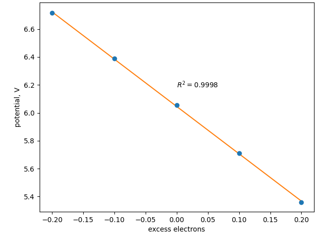
Due to the simple relationship between the excess electrons and the potential, reaching a desired potential is typically a fast process. If you are running a trajectory—for example, a relaxation, a molecular dynamics simulation, or a saddle-point search—the first image will often take a few repetitions (that is, sequential constant-electron calculations) until the desired potential is reached. Atoms typically move relatively little from image-to-image in a trajectory; therefore, subsequent images are often already at the target potential and no equilibration steps are necessary; when equilibration steps are required, the slope (of potential vs. number of electrons) is recalled from the last adjustment, and it often only takes a single equilibration step. Typically, over the course of a full trajectory, the added computational cost of working in the constant-potential ensemble is minimal, generally <50% greater computational time compared to a constant-charge calculation. As described in the Solvated Jellium Method (SJM) tutorial, this can sometimes be further improved by simultaneously optimizing the potential with the atomic positions.

References

[Kastlunger2018]

G. Kastlunger, P. Lindgren, A. A. Peterson, Controlled-Potential Simulation of Elementary Electrochemical Reactions: Proton Discharge on Metal Surfaces, J. Phys. Chem. C 122 (24), 12771 (2018)

[Held2014]

A. Held and M. Walter, Simplified continuum solvent model with a smooth cavity based on volumetric data, J. Chem. Phys. 141, 174108 (2014).

Class documentation

class gpaw.solvation.sjm.SJM(restart=None, **kwargs)

Solvated Jellium method. (Implemented as a subclass of the SolvationGPAW class.)

The method allows the simulation of an electrochemical environment, where the potential can be varied by changing the charging (that is, number of electrons) of the system. For this purpose, it allows the usagelof non- neutral periodic slab systems. Cell neutrality is achieved by adding a background charge in the solvent region above the slab

Further details are given in https://doi.org/10.1021/acs.jpcc.8b02465 If you use this method, we appreciate it if you cite that work.

The method can be run in two modes:

• Constant charge: The number of excess electrons in the simulation can be directly specified with the ‘excess_electrons’ keyword, leaving ‘target_potential’ set to None.

• Constant potential: The target potential (expressed as a work function) can be specified with the ‘target_potential’ keyword. Optionally, the ‘excess_electrons’ keyword can be supplied to specify the initial guess of the number of electrons.

By default, this method writes the grand-potential energy to the output; that is, the energy that has been adjusted with \(- \mu N\) (in this case, \(\mu\) is the work function and \(N\) is the excess electrons). This is the energy that is compatible with the forces in constant-potential mode and thus will behave well with optimizers, NEBs, etc. It is also frequently used in subsequent free-energy calculations.

Within this method, the potential is expressed as the top-side work function of the slab. Therefore, a potential of 0 V_SHE corresponds to a work function of roughly 4.4 eV. (That is, the user should specify target_potential as 4.4 in this case.) Because this method is attempting to bring the work function to a target value, the work function itself needs to be well-converged. For this reason, the ‘work function’ keyword is automatically added to the SCF convergence dictionary with a value of 0.001. This can be overriden by the user.

This method requires a dipole correction, and this is turned on automatically, but can be overridden with the poissonsolver keyword.

The SJM class takes a single argument, the sj dictionary. All other arguments are fed to the parent SolvationGPAW (and therefore GPAW) calculator.

Parameters:

sj: dict

Dictionary of parameters for the solvated jellium method, whose possible keys are given below.

Parameters in sj dictionary:

excess_electrons: float

Number of electrons added in the atomic system and (with opposite sign) in the background charge region. If the ‘target_potential’ keyword is also supplied, ‘excess_electrons’ is taken as an initial guess for the needed number of electrons.

target_potential: float

The potential that should be reached or kept in the course of the calculation. If set to ‘None’ (default) a constant-charge calculation based on the value of ‘excess_electrons’ is performed. Expressed as a work function, on the top side of the slab; see note above.

tol: float

Tolerance for the deviation of the target potential. If the potential is outside the defined range ‘ne’ will be changed in order to get inside again. Default: 0.01 V.

max_iters: int

In constant-potential mode, the maximum number of iterations to try to equilibrate the potential (by varying ne). Default: 10.

jelliumregion: dict

Parameters regarding the shape of the counter charge region. Implemented keys:

‘top’: float or None

Upper boundary of the counter charge region (z coordinate). A positive float is taken as the upper boundary coordiate. A negative float is taken as the distance below the uppper cell boundary. Default: -1.

‘bottom’: float or ‘cavity_like’ or None

Lower boundary of the counter-charge region (z coordinate). A positive float is taken as the lower boundary coordinate. A negative float is interpreted as the distance above the highest z coordinate of any atom; this can be fixed by setting fix_bottom to True. If ‘cavity_like’ is given the counter charge will take the form of the cavity up to the ‘top’. Default: -3.

‘thickness’: float or None

Thickness of the counter charge region in Angstroms. Can only be used if start is not ‘cavity_like’. Default: None

‘fix_bottom’: bool

Do not allow the lower limit of the jellium region to adapt to a change in the atomic geometry during a relaxation. Omitted in a ‘cavity_like’ jelliumregion. Default: False

grand_output: bool

Write the grand-potential energy into output files such as trajectory files. Default: True

always_adjust: bool

Adjust ne again even when potential is within tolerance. This is useful to set to True along with a loose potential tolerance (tol) to allow the potential and structure to be simultaneously optimized in a geometry optimization, for example. Default: False.

slopefloat or None

Initial guess of the slope, in volts per electron, of the relationship between the electrode potential and excess electrons, used to equilibrate the potential. This only applies to the first step, as the slope is calculated internally at subsequent steps. If None, will be guessed based on apparent capacitance of 10 uF/cm^2.

max_stepfloat

When equilibrating the potential, if a step results in the potential being further from the target and changing by more than ‘max_step’ V, then the step size is cut in half and we try again. This is to avoid leaving the linear region. You can set to np.inf to turn this off. Default: 2 V.

mixerfloat

Damping for the slope estimate. Because estimating slopes can sometimes be noisy (particularly for small changes, or when positions have also changed), some fraction of the previous slope estimate can be “mixed” with the current slope estimate before the new slope is established. E.g., new_slope = mixer * old_slope + (1. - mixer) * current_slope_estimate. Set to 0 for no damping. Default: 0.5.

Special SJM methods (in addition to those of GPAW/SolvationGPAW):

get_electrode_potential

Returns the potential of the simulated electrode, in V, relative to the vacuum.

write_sjm_traces

Write traces of quantities like electrostatic potential or cavity to disk.

Constructor for SolvationGPAW class.

Additional arguments not present in GPAW class: cavity – A Cavity instance. dielectric – A Dielectric instance. interactions – A list of Interaction instances.

class gpaw.solvation.sjm.SJMPower12Potential(atomic_radii=None, u0=0.18, pbc_cutoff=1e-06, tiny=1e-10, H2O_layer=False, unsolv_backside=True)

Inverse power-law potential. Inverse power law potential for SJM, inherited from the Power12Potential of gpaw.solvation. This is a 1/r^{12} repulive potential taking the value u0 at the atomic radius. In SJM one also has the option of removing the solvent from the electrode backside and adding ghost plane/atoms to remove the solvent from the electrode-water interface.

Parameters:

atomic_radii: function

Callable mapping an ase.Atoms object to an iterable of atomic radii in Angstroms. If not provided, defaults to van der Waals radii.

u0: float

Strength of the potential at the atomic radius in eV. Defaults to 0.18 eV, the best-fit value for water from Held & Walter.

pbc_cutoff: float

Cutoff in eV for including neighbor cells in a calculation with periodic boundary conditions.

H2O_layer: bool, int or str

True: Exclude the implicit solvent from the interface region between electrode and water. Ghost atoms will be added below the water layer. False: The opposite of True. [default] int: Explicitly account for the given number of water molecules above electrode. This is handy if H2O is directly adsorbed and a water layer is present in the unit cell at the same time. ‘plane’: Use a plane instead of ghost atoms for freeing the surface.

unsolv_backside: bool

Exclude implicit solvent from the region behind the electrode